View Jupyter notebook on the GitHub.
Prediction intervals#
![]()
This notebook contains overview of prediction intervals functionality in ETNA library.
Table of contents
Loading and preparing data
Estimating intervals using builtin method
Accessing prediction intervals in ``TSDataset` <#chapter2_1>`__
Computing interval metrics
Estimating prediction intervals using ``experimental.prediction_intervals` module <#chapter3>`__
`NaiveVariancePredictionIntervals<#chapter3_1>`__`ConformalPredictionIntervals<#chapter3_2>`__`EmpiricalPredictionIntervals<#chapter3_3>`__Prediction intervals for ensembles
Custom prediction interval method
Non-parametric method
Estimating historical residuals
[1]:
import warnings
from copy import deepcopy

import numpy as np
import pandas as pd

from etna.analysis.forecast import plot_forecast
from etna.datasets import TSDataset
from etna.metrics import Coverage
from etna.metrics import Width
from etna.models import CatBoostMultiSegmentModel
from etna.pipeline import Pipeline
from etna.transforms import DateFlagsTransform
from etna.transforms import LagTransform
from etna.transforms import SegmentEncoderTransform

warnings.filterwarnings("ignore")
[2]:
HORIZON = 30
Loading and preparing data#
Consider the dataset data/example_dataset.csv.
This data will be used to show how prediction intervals could be estimated and accessed in ETNA library.
The first step is to load data and convert it to the TSDataset.
[3]:
df = pd.read_csv("data/example_dataset.csv")
df = TSDataset.to_dataset(df=df)
ts = TSDataset(df=df, freq="D")

ts
[3]:
| segment | segment_a | segment_b | segment_c | segment_d |
|---|---|---|---|---|
| feature | target | target | target | target |
| timestamp | ||||
| 2019-01-01 | 170 | 102 | 92 | 238 |
| 2019-01-02 | 243 | 123 | 107 | 358 |
| 2019-01-03 | 267 | 130 | 103 | 366 |
| 2019-01-04 | 287 | 138 | 103 | 385 |
| 2019-01-05 | 279 | 137 | 104 | 384 |
| ... | ... | ... | ... | ... |
| 2019-11-26 | 591 | 259 | 196 | 941 |
| 2019-11-27 | 606 | 264 | 196 | 949 |
| 2019-11-28 | 555 | 242 | 207 | 896 |
| 2019-11-29 | 581 | 247 | 186 | 905 |
| 2019-11-30 | 502 | 206 | 169 | 721 |
334 rows × 4 columns
[4]:
ts.plot()
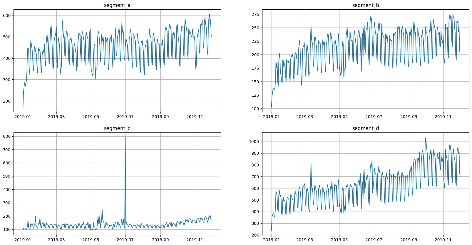
Here we have four segments in the dataset. All segments have seasonalities, and some of them show signs of trend. Note that segment C contains an obvious outlier, that may affect quality of estimated intervals.
In the next step, we split our dataset into two parts: train and test. The test part will be used as a hold-out dataset for metrics computation and result analysis.
[5]:
train_ts, test_ts = ts.train_test_split(test_size=HORIZON)
Estimating intervals using builtin method#
Prediction interval is an estimation of the range in which a future observation will fall, with a certain probability, given historical observations.
There are several ways of estimation: model-specific and model-agnostic methods. Model-specific methods use features of underlying models, that are able to produce probabilistic estimates. Examples of such models are SARIMAX, Holt-Winters and TBATS. Model-agnostic methods treat models as black boxes and implement separate methods to do the estimation. The topic of this notebook is model-agnostic methods only.
Currently there are several types of prediction intervals in the library: 1. Quantiles estimates 2. Arbitrary interval borders, that tend to provide desired coverage
Quantiles estimation methods, implemented in the library, use univariate distribution to estimate quantiles at each timestamp in the horizon. There is the possibility of treating all timestamps in the horizon jointly as multivariate random variable to estimate quantiles, but this approach is not implemented right now. The extension of current method pool will be discussed in the last section of this notebook.
So there are some naming convention to achieve distinction between two types of intervals. Borders that approximate quantiles named using the following format {target_{q:.4g}}, where q is the corresponding quantile level. And there are no particular rules for the arbitrary borders. But it is implementation responsibility to name them appropriately.
Before estimating prediction intervals we need to fit a model. Here CatBoostMultiSegmentModel is used with lag and date features. This model requires computed features, so we add corresponding transforms to the pipeline.
[6]:
seg = SegmentEncoderTransform()
lags = LagTransform(in_column="target", lags=list(range(HORIZON, 20 + HORIZON)), out_column="lag")
date_flags = DateFlagsTransform(
    day_number_in_week=True,
    day_number_in_month=True,
    week_number_in_month=True,
    week_number_in_year=True,
    month_number_in_year=True,
    year_number=True,
    is_weekend=True,
    out_column="flag",
)

transforms = [lags, date_flags, seg]
[7]:
model = CatBoostMultiSegmentModel()
[8]:
pipeline = Pipeline(model=model, transforms=transforms, horizon=HORIZON)

pipeline.fit(ts=train_ts);
After the pipeline is defined and fitted, we are able to estimate prediction intervals with the default method. To do so set the prediction_interval=True parameter of the forecast method.
This method is based on residual variance estimation and \(z\)-scores. Variance estimation is done via running historical backtest on non-overlapping folds. Number of folds is controlled by the n_folds parameter.
[9]:
forecast = pipeline.forecast(ts=train_ts, prediction_interval=True, n_folds=7)
forecast
[Parallel(n_jobs=1)]: Using backend SequentialBackend with 1 concurrent workers.
[Parallel(n_jobs=1)]: Done   1 out of   1 | elapsed:    5.8s remaining:    0.0s
[Parallel(n_jobs=1)]: Done   2 out of   2 | elapsed:   10.4s remaining:    0.0s
[Parallel(n_jobs=1)]: Done   3 out of   3 | elapsed:   16.0s remaining:    0.0s
[Parallel(n_jobs=1)]: Done   4 out of   4 | elapsed:   22.3s remaining:    0.0s
[Parallel(n_jobs=1)]: Done   5 out of   5 | elapsed:   27.9s remaining:    0.0s
[Parallel(n_jobs=1)]: Done   6 out of   6 | elapsed:   33.9s remaining:    0.0s
[Parallel(n_jobs=1)]: Done   7 out of   7 | elapsed:   39.6s remaining:    0.0s
[Parallel(n_jobs=1)]: Done   7 out of   7 | elapsed:   39.6s finished
[Parallel(n_jobs=1)]: Using backend SequentialBackend with 1 concurrent workers.
[Parallel(n_jobs=1)]: Done   1 out of   1 | elapsed:    0.1s remaining:    0.0s
[Parallel(n_jobs=1)]: Done   2 out of   2 | elapsed:    0.3s remaining:    0.0s
[Parallel(n_jobs=1)]: Done   3 out of   3 | elapsed:    0.4s remaining:    0.0s
[Parallel(n_jobs=1)]: Done   4 out of   4 | elapsed:    0.6s remaining:    0.0s
[Parallel(n_jobs=1)]: Done   5 out of   5 | elapsed:    0.7s remaining:    0.0s
[Parallel(n_jobs=1)]: Done   6 out of   6 | elapsed:    0.9s remaining:    0.0s
[Parallel(n_jobs=1)]: Done   7 out of   7 | elapsed:    1.0s remaining:    0.0s
[Parallel(n_jobs=1)]: Done   7 out of   7 | elapsed:    1.0s finished
[Parallel(n_jobs=1)]: Using backend SequentialBackend with 1 concurrent workers.
[Parallel(n_jobs=1)]: Done   1 out of   1 | elapsed:    0.0s remaining:    0.0s
[Parallel(n_jobs=1)]: Done   2 out of   2 | elapsed:    0.1s remaining:    0.0s
[Parallel(n_jobs=1)]: Done   3 out of   3 | elapsed:    0.1s remaining:    0.0s
[Parallel(n_jobs=1)]: Done   4 out of   4 | elapsed:    0.2s remaining:    0.0s
[Parallel(n_jobs=1)]: Done   5 out of   5 | elapsed:    0.2s remaining:    0.0s
[Parallel(n_jobs=1)]: Done   6 out of   6 | elapsed:    0.2s remaining:    0.0s
[Parallel(n_jobs=1)]: Done   7 out of   7 | elapsed:    0.2s remaining:    0.0s
[Parallel(n_jobs=1)]: Done   7 out of   7 | elapsed:    0.2s finished
[9]:
| segment | segment_a | ... | segment_d | ||||||||||||||||||
|---|---|---|---|---|---|---|---|---|---|---|---|---|---|---|---|---|---|---|---|---|---|
| feature | flag_day_number_in_month | flag_day_number_in_week | flag_is_weekend | flag_month_number_in_year | flag_week_number_in_month | flag_week_number_in_year | flag_year_number | lag_30 | lag_31 | lag_32 | ... | lag_44 | lag_45 | lag_46 | lag_47 | lag_48 | lag_49 | segment_code | target | target_0.025 | target_0.975 |
| timestamp | |||||||||||||||||||||
| 2019-11-01 | 1 | 4 | False | 11 | 1 | 44 | 2019 | 516.0 | 558.0 | 551.0 | ... | 860.0 | 859.0 | 833.0 | 592.0 | 616.0 | 824.0 | 3 | 884.890130 | 733.931966 | 1035.848293 |
| 2019-11-02 | 2 | 5 | True | 11 | 1 | 44 | 2019 | 489.0 | 516.0 | 558.0 | ... | 822.0 | 860.0 | 859.0 | 833.0 | 592.0 | 616.0 | 3 | 766.540795 | 615.582631 | 917.498959 |
| 2019-11-03 | 3 | 6 | True | 11 | 1 | 44 | 2019 | 471.0 | 489.0 | 516.0 | ... | 908.0 | 822.0 | 860.0 | 859.0 | 833.0 | 592.0 | 3 | 735.275270 | 584.317106 | 886.233433 |
| 2019-11-04 | 4 | 0 | False | 11 | 2 | 45 | 2019 | 371.0 | 471.0 | 489.0 | ... | 648.0 | 908.0 | 822.0 | 860.0 | 859.0 | 833.0 | 3 | 871.086070 | 720.127906 | 1022.044233 |
| 2019-11-05 | 5 | 1 | False | 11 | 2 | 45 | 2019 | 359.0 | 371.0 | 471.0 | ... | 599.0 | 648.0 | 908.0 | 822.0 | 860.0 | 859.0 | 3 | 854.657442 | 703.699278 | 1005.615606 |
| 2019-11-06 | 6 | 2 | False | 11 | 2 | 45 | 2019 | 499.0 | 359.0 | 371.0 | ... | 821.0 | 599.0 | 648.0 | 908.0 | 822.0 | 860.0 | 3 | 845.998526 | 695.040362 | 996.956690 |
| 2019-11-07 | 7 | 3 | False | 11 | 2 | 45 | 2019 | 528.0 | 499.0 | 359.0 | ... | 883.0 | 821.0 | 599.0 | 648.0 | 908.0 | 822.0 | 3 | 863.000343 | 712.042180 | 1013.958507 |
| 2019-11-08 | 8 | 4 | False | 11 | 2 | 45 | 2019 | 550.0 | 528.0 | 499.0 | ... | 923.0 | 883.0 | 821.0 | 599.0 | 648.0 | 908.0 | 3 | 886.018643 | 735.060480 | 1036.976807 |
| 2019-11-09 | 9 | 5 | True | 11 | 2 | 45 | 2019 | 547.0 | 550.0 | 528.0 | ... | 908.0 | 923.0 | 883.0 | 821.0 | 599.0 | 648.0 | 3 | 786.671129 | 635.712965 | 937.629293 |
| 2019-11-10 | 10 | 6 | True | 11 | 2 | 45 | 2019 | 544.0 | 547.0 | 550.0 | ... | 874.0 | 908.0 | 923.0 | 883.0 | 821.0 | 599.0 | 3 | 770.142993 | 619.184829 | 921.101157 |
| 2019-11-11 | 11 | 0 | False | 11 | 3 | 46 | 2019 | 423.0 | 544.0 | 547.0 | ... | 712.0 | 874.0 | 908.0 | 923.0 | 883.0 | 821.0 | 3 | 883.026096 | 732.067932 | 1033.984259 |
| 2019-11-12 | 12 | 1 | False | 11 | 3 | 46 | 2019 | 402.0 | 423.0 | 544.0 | ... | 691.0 | 712.0 | 874.0 | 908.0 | 923.0 | 883.0 | 3 | 867.552488 | 716.594324 | 1018.510651 |
| 2019-11-13 | 13 | 2 | False | 11 | 3 | 46 | 2019 | 550.0 | 402.0 | 423.0 | ... | 980.0 | 691.0 | 712.0 | 874.0 | 908.0 | 923.0 | 3 | 850.850720 | 699.892556 | 1001.808883 |
| 2019-11-14 | 14 | 3 | False | 11 | 3 | 46 | 2019 | 582.0 | 550.0 | 402.0 | ... | 1037.0 | 980.0 | 691.0 | 712.0 | 874.0 | 908.0 | 3 | 866.155902 | 715.197738 | 1017.114066 |
| 2019-11-15 | 15 | 4 | False | 11 | 3 | 46 | 2019 | 559.0 | 582.0 | 550.0 | ... | 969.0 | 1037.0 | 980.0 | 691.0 | 712.0 | 874.0 | 3 | 891.686379 | 740.728216 | 1042.644543 |
| 2019-11-16 | 16 | 5 | True | 11 | 3 | 46 | 2019 | 543.0 | 559.0 | 582.0 | ... | 929.0 | 969.0 | 1037.0 | 980.0 | 691.0 | 712.0 | 3 | 795.462403 | 644.504240 | 946.420567 |
| 2019-11-17 | 17 | 6 | True | 11 | 3 | 46 | 2019 | 523.0 | 543.0 | 559.0 | ... | 874.0 | 929.0 | 969.0 | 1037.0 | 980.0 | 691.0 | 3 | 794.104098 | 643.145934 | 945.062262 |
| 2019-11-18 | 18 | 0 | False | 11 | 4 | 47 | 2019 | 422.0 | 523.0 | 543.0 | ... | 664.0 | 874.0 | 929.0 | 969.0 | 1037.0 | 980.0 | 3 | 869.079738 | 718.121574 | 1020.037902 |
| 2019-11-19 | 19 | 1 | False | 11 | 4 | 47 | 2019 | 403.0 | 422.0 | 523.0 | ... | 623.0 | 664.0 | 874.0 | 929.0 | 969.0 | 1037.0 | 3 | 855.177747 | 704.219583 | 1006.135911 |
| 2019-11-20 | 20 | 2 | False | 11 | 4 | 47 | 2019 | 538.0 | 403.0 | 422.0 | ... | 841.0 | 623.0 | 664.0 | 874.0 | 929.0 | 969.0 | 3 | 850.930059 | 699.971896 | 1001.888223 |
| 2019-11-21 | 21 | 3 | False | 11 | 4 | 47 | 2019 | 532.0 | 538.0 | 403.0 | ... | 879.0 | 841.0 | 623.0 | 664.0 | 874.0 | 929.0 | 3 | 870.278782 | 719.320619 | 1021.236946 |
| 2019-11-22 | 22 | 4 | False | 11 | 4 | 47 | 2019 | 515.0 | 532.0 | 538.0 | ... | 886.0 | 879.0 | 841.0 | 623.0 | 664.0 | 874.0 | 3 | 890.245006 | 739.286843 | 1041.203170 |
| 2019-11-23 | 23 | 5 | True | 11 | 4 | 47 | 2019 | 520.0 | 515.0 | 532.0 | ... | 934.0 | 886.0 | 879.0 | 841.0 | 623.0 | 664.0 | 3 | 775.886589 | 624.928425 | 926.844753 |
| 2019-11-24 | 24 | 6 | True | 11 | 4 | 47 | 2019 | 511.0 | 520.0 | 515.0 | ... | 885.0 | 934.0 | 886.0 | 879.0 | 841.0 | 623.0 | 3 | 751.033775 | 600.075611 | 901.991938 |
| 2019-11-25 | 25 | 0 | False | 11 | 5 | 48 | 2019 | 502.0 | 511.0 | 520.0 | ... | 672.0 | 885.0 | 934.0 | 886.0 | 879.0 | 841.0 | 3 | 874.921950 | 723.963786 | 1025.880114 |
| 2019-11-26 | 26 | 1 | False | 11 | 5 | 48 | 2019 | 499.0 | 502.0 | 511.0 | ... | 621.0 | 672.0 | 885.0 | 934.0 | 886.0 | 879.0 | 3 | 878.395149 | 727.436985 | 1029.353313 |
| 2019-11-27 | 27 | 2 | False | 11 | 5 | 48 | 2019 | 534.0 | 499.0 | 502.0 | ... | 859.0 | 621.0 | 672.0 | 885.0 | 934.0 | 886.0 | 3 | 860.259958 | 709.301795 | 1011.218122 |
| 2019-11-28 | 28 | 3 | False | 11 | 5 | 48 | 2019 | 502.0 | 534.0 | 499.0 | ... | 931.0 | 859.0 | 621.0 | 672.0 | 885.0 | 934.0 | 3 | 889.115142 | 738.156978 | 1040.073305 |
| 2019-11-29 | 29 | 4 | False | 11 | 5 | 48 | 2019 | 497.0 | 502.0 | 534.0 | ... | 897.0 | 931.0 | 859.0 | 621.0 | 672.0 | 885.0 | 3 | 891.706478 | 740.748315 | 1042.664642 |
| 2019-11-30 | 30 | 5 | True | 11 | 5 | 48 | 2019 | 501.0 | 497.0 | 502.0 | ... | 882.0 | 897.0 | 931.0 | 859.0 | 621.0 | 672.0 | 3 | 779.465792 | 628.507628 | 930.423955 |
30 rows × 124 columns
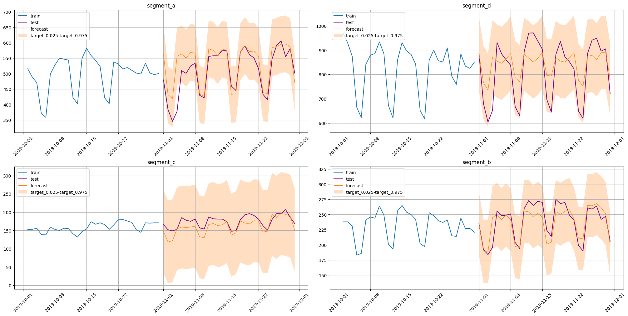
Here we have a point forecast for the full horizon, along with an estimated prediction interval for each segment.
The section below describes how one can perform manipulations with intervals in the dataset with forecasts.
Accessing prediction intervals in TSDataset#
Column names for the estimated prediction intervals can be obtained using the TSDataset.prediction_intervals_names property.
[10]:
forecast.prediction_intervals_names
[10]:
('target_0.025', 'target_0.975')
Here segment names are omitted, because they share interval estimation method. So column names identical for all the segments.
A dataframe with prediction intervals for each segment can be obtained by using the TSDataset.get_prediction_intervals() method.
Here, we save such dataframe to a separate object to use later.
[11]:
prediction_intervals = forecast.get_prediction_intervals()
prediction_intervals
[11]:
| segment | segment_a | segment_b | segment_c | segment_d | ||||
|---|---|---|---|---|---|---|---|---|
| feature | target_0.025 | target_0.975 | target_0.025 | target_0.975 | target_0.025 | target_0.975 | target_0.025 | target_0.975 |
| timestamp | ||||||||
| 2019-11-01 | 470.753353 | 654.622675 | 182.998175 | 287.116897 | 33.867819 | 260.423229 | 733.931966 | 1035.848293 |
| 2019-11-02 | 339.787734 | 523.657056 | 137.674295 | 241.793017 | 5.273997 | 231.829407 | 615.582631 | 917.498959 |
| 2019-11-03 | 328.057195 | 511.926517 | 136.459431 | 240.578153 | 8.896867 | 235.452277 | 584.317106 | 886.233433 |
| 2019-11-04 | 464.257076 | 648.126398 | 193.140438 | 297.259160 | 41.574061 | 268.129472 | 720.127906 | 1022.044233 |
| 2019-11-05 | 471.667537 | 655.536859 | 197.889160 | 302.007882 | 46.067009 | 272.622419 | 703.699278 | 1005.615606 |
| 2019-11-06 | 458.729249 | 642.598571 | 189.420442 | 293.539164 | 44.816511 | 271.371921 | 695.040362 | 996.956690 |
| 2019-11-07 | 477.280688 | 661.150010 | 197.562499 | 301.681221 | 46.092846 | 272.648256 | 712.042180 | 1013.958507 |
| 2019-11-08 | 474.032182 | 657.901504 | 189.213408 | 293.332130 | 48.396520 | 274.951930 | 735.060480 | 1036.976807 |
| 2019-11-09 | 342.156468 | 526.025790 | 145.463552 | 249.582274 | 19.344079 | 245.899489 | 635.712965 | 937.629293 |
| 2019-11-10 | 335.175499 | 519.044821 | 143.336403 | 247.455125 | 17.194591 | 243.750001 | 619.184829 | 921.101157 |
| 2019-11-11 | 488.455591 | 672.324913 | 202.226734 | 306.345456 | 52.974858 | 279.530268 | 732.067932 | 1033.984259 |
| 2019-11-12 | 483.315864 | 667.185186 | 203.543648 | 307.662371 | 55.758080 | 282.313490 | 716.594324 | 1018.510651 |
| 2019-11-13 | 466.986283 | 650.855605 | 194.021186 | 298.139908 | 50.141150 | 276.696560 | 699.892556 | 1001.808883 |
| 2019-11-14 | 487.949334 | 671.818656 | 199.896469 | 304.015191 | 52.315531 | 278.870942 | 715.197738 | 1017.114066 |
| 2019-11-15 | 482.792684 | 666.662006 | 193.939262 | 298.057985 | 61.206762 | 287.762172 | 740.728216 | 1042.644543 |
| 2019-11-16 | 341.268023 | 525.137344 | 149.079266 | 253.197988 | 23.712223 | 250.267633 | 644.504240 | 946.420567 |
| 2019-11-17 | 342.778361 | 526.647683 | 152.365006 | 256.483728 | 30.379443 | 256.934853 | 643.145934 | 945.062262 |
| 2019-11-18 | 479.061701 | 662.931023 | 202.628841 | 306.747563 | 62.492294 | 289.047705 | 718.121574 | 1020.037902 |
| 2019-11-19 | 499.022561 | 682.891883 | 198.347958 | 302.466681 | 57.142646 | 283.698056 | 704.219583 | 1006.135911 |
| 2019-11-20 | 479.542225 | 663.411547 | 203.284886 | 307.403608 | 54.747406 | 281.302817 | 699.971896 | 1001.888223 |
| 2019-11-21 | 481.230732 | 665.100054 | 205.877484 | 309.996207 | 63.412175 | 289.967586 | 719.320619 | 1021.236946 |
| 2019-11-22 | 464.535473 | 648.404795 | 190.887708 | 295.006430 | 62.151579 | 288.706989 | 739.286843 | 1041.203170 |
| 2019-11-23 | 346.853867 | 530.723188 | 159.171331 | 263.290053 | 32.471348 | 259.026758 | 624.928425 | 926.844753 |
| 2019-11-24 | 343.750821 | 527.620143 | 157.939006 | 262.057728 | 34.721080 | 261.276491 | 600.075611 | 901.991938 |
| 2019-11-25 | 492.355361 | 676.224683 | 212.837537 | 316.956260 | 80.679910 | 307.235320 | 723.963786 | 1025.880114 |
| 2019-11-26 | 495.916553 | 679.785875 | 212.490423 | 316.609145 | 72.072010 | 298.627420 | 727.436985 | 1029.353313 |
| 2019-11-27 | 503.081899 | 686.951221 | 216.030382 | 320.149104 | 83.249364 | 309.804775 | 709.301795 | 1011.218122 |
| 2019-11-28 | 504.440254 | 688.309575 | 209.345608 | 313.464330 | 80.577678 | 307.133088 | 738.156978 | 1040.073305 |
| 2019-11-29 | 495.299379 | 679.168701 | 199.689472 | 303.808194 | 76.070869 | 302.626279 | 740.748315 | 1042.664642 |
| 2019-11-30 | 379.529016 | 563.398338 | 148.540798 | 252.659521 | 37.882227 | 264.437637 | 628.507628 | 930.423955 |
If estimated intervals are no longer needed or there is a necessity to remove prediction intervals from the dataset use TSDataset.drop_prediction_intervals() method.
[12]:
forecast.drop_prediction_intervals()
forecast.prediction_intervals_names
[12]:
()
Here we see that property contains an empty tuple now. It is an indication that no intervals are registered.
[13]:
forecast.get_prediction_intervals()
Calling TSDataset.get_prediction_intervals() in such a case will return None.
There is a possibility of adding existing prediction intervals to the dataset. To do so, one should use TSDataset.add_prediction_intervals() method.
There are a couple requirements when adding existing intervals to the dataset. 1. Absence of the intervals in the dataset. This could be checked via the prediction_intervals_names property. 2. The dataframe with intervals should be in ETNA wide format. 3. All segments should be matched between the dataset and intervals dataframe. 4. Interval borders names are matched across all the segments.
[14]:
forecast.add_prediction_intervals(prediction_intervals_df=prediction_intervals)
forecast.prediction_intervals_names
[14]:
('target_0.025', 'target_0.975')
[15]:
forecast
[15]:
| segment | segment_a | ... | segment_d | ||||||||||||||||||
|---|---|---|---|---|---|---|---|---|---|---|---|---|---|---|---|---|---|---|---|---|---|
| feature | flag_day_number_in_month | flag_day_number_in_week | flag_is_weekend | flag_month_number_in_year | flag_week_number_in_month | flag_week_number_in_year | flag_year_number | lag_30 | lag_31 | lag_32 | ... | lag_44 | lag_45 | lag_46 | lag_47 | lag_48 | lag_49 | segment_code | target | target_0.025 | target_0.975 |
| timestamp | |||||||||||||||||||||
| 2019-11-01 | 1 | 4 | False | 11 | 1 | 44 | 2019 | 516.0 | 558.0 | 551.0 | ... | 860.0 | 859.0 | 833.0 | 592.0 | 616.0 | 824.0 | 3 | 884.890130 | 733.931966 | 1035.848293 |
| 2019-11-02 | 2 | 5 | True | 11 | 1 | 44 | 2019 | 489.0 | 516.0 | 558.0 | ... | 822.0 | 860.0 | 859.0 | 833.0 | 592.0 | 616.0 | 3 | 766.540795 | 615.582631 | 917.498959 |
| 2019-11-03 | 3 | 6 | True | 11 | 1 | 44 | 2019 | 471.0 | 489.0 | 516.0 | ... | 908.0 | 822.0 | 860.0 | 859.0 | 833.0 | 592.0 | 3 | 735.275270 | 584.317106 | 886.233433 |
| 2019-11-04 | 4 | 0 | False | 11 | 2 | 45 | 2019 | 371.0 | 471.0 | 489.0 | ... | 648.0 | 908.0 | 822.0 | 860.0 | 859.0 | 833.0 | 3 | 871.086070 | 720.127906 | 1022.044233 |
| 2019-11-05 | 5 | 1 | False | 11 | 2 | 45 | 2019 | 359.0 | 371.0 | 471.0 | ... | 599.0 | 648.0 | 908.0 | 822.0 | 860.0 | 859.0 | 3 | 854.657442 | 703.699278 | 1005.615606 |
| 2019-11-06 | 6 | 2 | False | 11 | 2 | 45 | 2019 | 499.0 | 359.0 | 371.0 | ... | 821.0 | 599.0 | 648.0 | 908.0 | 822.0 | 860.0 | 3 | 845.998526 | 695.040362 | 996.956690 |
| 2019-11-07 | 7 | 3 | False | 11 | 2 | 45 | 2019 | 528.0 | 499.0 | 359.0 | ... | 883.0 | 821.0 | 599.0 | 648.0 | 908.0 | 822.0 | 3 | 863.000343 | 712.042180 | 1013.958507 |
| 2019-11-08 | 8 | 4 | False | 11 | 2 | 45 | 2019 | 550.0 | 528.0 | 499.0 | ... | 923.0 | 883.0 | 821.0 | 599.0 | 648.0 | 908.0 | 3 | 886.018643 | 735.060480 | 1036.976807 |
| 2019-11-09 | 9 | 5 | True | 11 | 2 | 45 | 2019 | 547.0 | 550.0 | 528.0 | ... | 908.0 | 923.0 | 883.0 | 821.0 | 599.0 | 648.0 | 3 | 786.671129 | 635.712965 | 937.629293 |
| 2019-11-10 | 10 | 6 | True | 11 | 2 | 45 | 2019 | 544.0 | 547.0 | 550.0 | ... | 874.0 | 908.0 | 923.0 | 883.0 | 821.0 | 599.0 | 3 | 770.142993 | 619.184829 | 921.101157 |
| 2019-11-11 | 11 | 0 | False | 11 | 3 | 46 | 2019 | 423.0 | 544.0 | 547.0 | ... | 712.0 | 874.0 | 908.0 | 923.0 | 883.0 | 821.0 | 3 | 883.026096 | 732.067932 | 1033.984259 |
| 2019-11-12 | 12 | 1 | False | 11 | 3 | 46 | 2019 | 402.0 | 423.0 | 544.0 | ... | 691.0 | 712.0 | 874.0 | 908.0 | 923.0 | 883.0 | 3 | 867.552488 | 716.594324 | 1018.510651 |
| 2019-11-13 | 13 | 2 | False | 11 | 3 | 46 | 2019 | 550.0 | 402.0 | 423.0 | ... | 980.0 | 691.0 | 712.0 | 874.0 | 908.0 | 923.0 | 3 | 850.850720 | 699.892556 | 1001.808883 |
| 2019-11-14 | 14 | 3 | False | 11 | 3 | 46 | 2019 | 582.0 | 550.0 | 402.0 | ... | 1037.0 | 980.0 | 691.0 | 712.0 | 874.0 | 908.0 | 3 | 866.155902 | 715.197738 | 1017.114066 |
| 2019-11-15 | 15 | 4 | False | 11 | 3 | 46 | 2019 | 559.0 | 582.0 | 550.0 | ... | 969.0 | 1037.0 | 980.0 | 691.0 | 712.0 | 874.0 | 3 | 891.686379 | 740.728216 | 1042.644543 |
| 2019-11-16 | 16 | 5 | True | 11 | 3 | 46 | 2019 | 543.0 | 559.0 | 582.0 | ... | 929.0 | 969.0 | 1037.0 | 980.0 | 691.0 | 712.0 | 3 | 795.462403 | 644.504240 | 946.420567 |
| 2019-11-17 | 17 | 6 | True | 11 | 3 | 46 | 2019 | 523.0 | 543.0 | 559.0 | ... | 874.0 | 929.0 | 969.0 | 1037.0 | 980.0 | 691.0 | 3 | 794.104098 | 643.145934 | 945.062262 |
| 2019-11-18 | 18 | 0 | False | 11 | 4 | 47 | 2019 | 422.0 | 523.0 | 543.0 | ... | 664.0 | 874.0 | 929.0 | 969.0 | 1037.0 | 980.0 | 3 | 869.079738 | 718.121574 | 1020.037902 |
| 2019-11-19 | 19 | 1 | False | 11 | 4 | 47 | 2019 | 403.0 | 422.0 | 523.0 | ... | 623.0 | 664.0 | 874.0 | 929.0 | 969.0 | 1037.0 | 3 | 855.177747 | 704.219583 | 1006.135911 |
| 2019-11-20 | 20 | 2 | False | 11 | 4 | 47 | 2019 | 538.0 | 403.0 | 422.0 | ... | 841.0 | 623.0 | 664.0 | 874.0 | 929.0 | 969.0 | 3 | 850.930059 | 699.971896 | 1001.888223 |
| 2019-11-21 | 21 | 3 | False | 11 | 4 | 47 | 2019 | 532.0 | 538.0 | 403.0 | ... | 879.0 | 841.0 | 623.0 | 664.0 | 874.0 | 929.0 | 3 | 870.278782 | 719.320619 | 1021.236946 |
| 2019-11-22 | 22 | 4 | False | 11 | 4 | 47 | 2019 | 515.0 | 532.0 | 538.0 | ... | 886.0 | 879.0 | 841.0 | 623.0 | 664.0 | 874.0 | 3 | 890.245006 | 739.286843 | 1041.203170 |
| 2019-11-23 | 23 | 5 | True | 11 | 4 | 47 | 2019 | 520.0 | 515.0 | 532.0 | ... | 934.0 | 886.0 | 879.0 | 841.0 | 623.0 | 664.0 | 3 | 775.886589 | 624.928425 | 926.844753 |
| 2019-11-24 | 24 | 6 | True | 11 | 4 | 47 | 2019 | 511.0 | 520.0 | 515.0 | ... | 885.0 | 934.0 | 886.0 | 879.0 | 841.0 | 623.0 | 3 | 751.033775 | 600.075611 | 901.991938 |
| 2019-11-25 | 25 | 0 | False | 11 | 5 | 48 | 2019 | 502.0 | 511.0 | 520.0 | ... | 672.0 | 885.0 | 934.0 | 886.0 | 879.0 | 841.0 | 3 | 874.921950 | 723.963786 | 1025.880114 |
| 2019-11-26 | 26 | 1 | False | 11 | 5 | 48 | 2019 | 499.0 | 502.0 | 511.0 | ... | 621.0 | 672.0 | 885.0 | 934.0 | 886.0 | 879.0 | 3 | 878.395149 | 727.436985 | 1029.353313 |
| 2019-11-27 | 27 | 2 | False | 11 | 5 | 48 | 2019 | 534.0 | 499.0 | 502.0 | ... | 859.0 | 621.0 | 672.0 | 885.0 | 934.0 | 886.0 | 3 | 860.259958 | 709.301795 | 1011.218122 |
| 2019-11-28 | 28 | 3 | False | 11 | 5 | 48 | 2019 | 502.0 | 534.0 | 499.0 | ... | 931.0 | 859.0 | 621.0 | 672.0 | 885.0 | 934.0 | 3 | 889.115142 | 738.156978 | 1040.073305 |
| 2019-11-29 | 29 | 4 | False | 11 | 5 | 48 | 2019 | 497.0 | 502.0 | 534.0 | ... | 897.0 | 931.0 | 859.0 | 621.0 | 672.0 | 885.0 | 3 | 891.706478 | 740.748315 | 1042.664642 |
| 2019-11-30 | 30 | 5 | True | 11 | 5 | 48 | 2019 | 501.0 | 497.0 | 502.0 | ... | 882.0 | 897.0 | 931.0 | 859.0 | 621.0 | 672.0 | 3 | 779.465792 | 628.507628 | 930.423955 |
30 rows × 124 columns
We called prediction_intervals_names here to ensure that intervals were correctly added and printed out the resulting dataset.
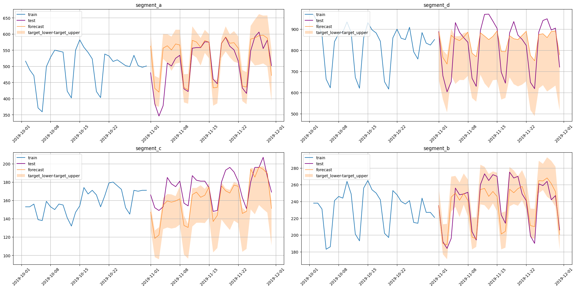
Results visualization could be done using the plot_forecast function. Setting parameter prediction_intervals=True will enable plotting estimated prediction intervals.
[16]:
plot_forecast(forecast, test_ts, train_ts, prediction_intervals=True, n_train_samples=30)
Computing interval metrics#
There are a couple of metrics in the library that can help estimate the quality of computed prediction intervals: * Coverage - percentage of points in the horizon that fall between interval borders * Width - mean distance between intervals borders at each timestamp of the horizon.
These metrics require initialization. To specify which interval to use provide border names by setting lower_name and upper_name parameters. After initialization these metrics will try to find specified borders in the dataset with predicted values. If provided names are not found, a corresponding error will be raised.
If estimated intervals borders are quantiles desired levels could be selected by setting the quantiles parameter. Usage of both ways of interval selection will lead to an error.
Here we wrap metrics estimation in one function.
[17]:
def interval_metrics(test_ts, forecast):
    lower_name, upper_name = forecast.prediction_intervals_names

    coverage = Coverage(lower_name=lower_name, upper_name=upper_name)(test_ts, forecast)
    width = Width(lower_name=lower_name, upper_name=upper_name)(test_ts, forecast)

    return coverage, width
[18]:
coverage, width = interval_metrics(test_ts=test_ts, forecast=forecast)
[19]:
coverage
[19]:
{'segment_a': 0.9666666666666667,
 'segment_b': 1.0,
 'segment_c': 1.0,
 'segment_d': 0.9666666666666667}
[20]:
width
[20]:
{'segment_a': 183.8693219098439,
 'segment_b': 104.11872216880786,
 'segment_c': 226.55541023779915,
 'segment_d': 301.9163274096744}
Estimating prediction intervals using experimental.prediction_intervals module#
The ETNA library provides several alternative methods for prediction interval estimation. All necessary functionality is in the etna.experimental.prediction_intervals module.
This section covers currently implemented methods. Also, the module provides the possibility to easily extend the method list by implementing a custom one. This topic will be discussed in the last section.
Prediction interval functionality is implemented via wrapper classes for the ETNA pipelines. During initialization, such methods require pipeline instances and necessary hyperparameters. Provided pipeline can be fitted before or after wrapping with the interval estimation method.
NaiveVariancePredictionIntervals#
This method estimates prediction quantiles using the following algorithm:
Compute the residuals matrix \(r_{it} = \hat y_{it} - y_{it}\) using k-fold backtest, where \(i\) is fold index.
Estimate variance for each step in the prediction horizon \(v_t = \frac{1}{k} \sum_{i = 1}^k r_{it}^2\).
Use \(z\)-scores and estimated variance to compute corresponding quantiles.
Desired quantiles levels for the prediction interval can be set via quantiles of the forecast method.
[21]:
from etna.experimental.prediction_intervals import NaiveVariancePredictionIntervals
pipeline = NaiveVariancePredictionIntervals(pipeline=pipeline)
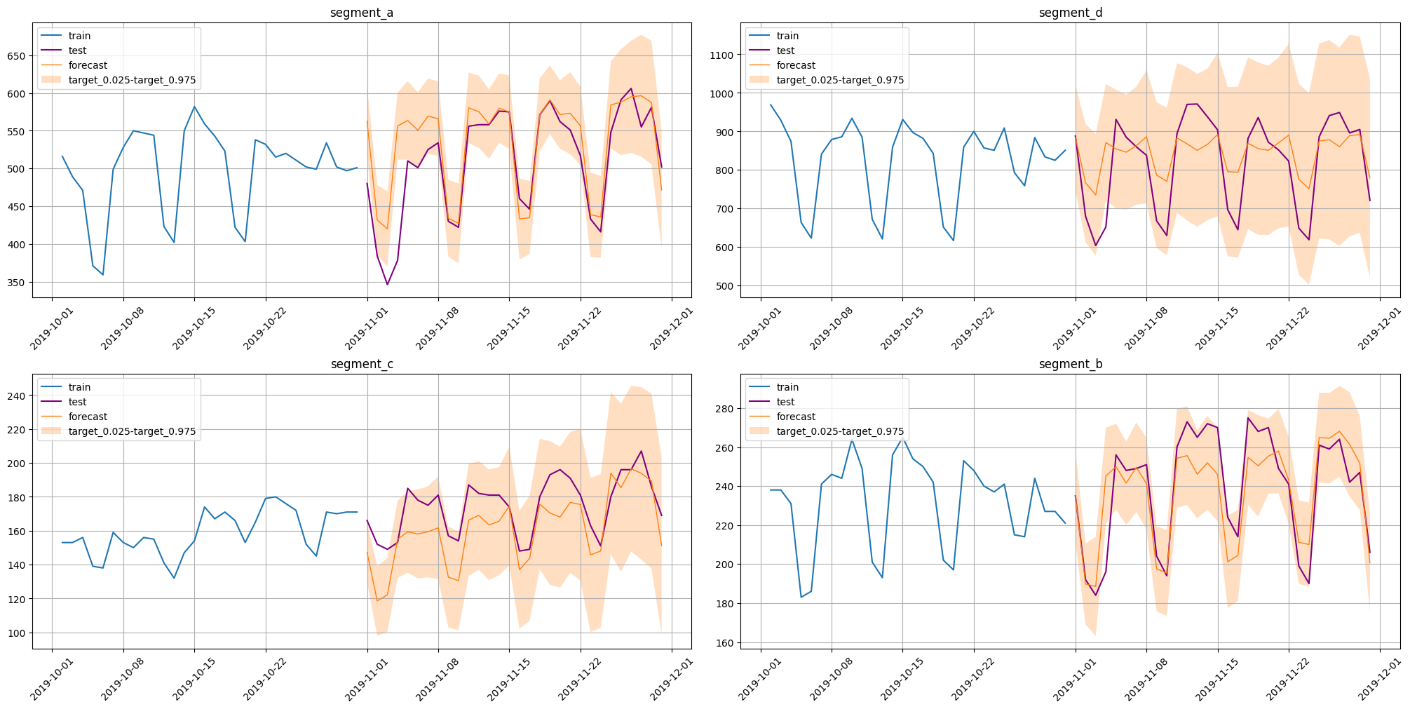
forecast = pipeline.forecast(quantiles=(0.025, 0.975), prediction_interval=True, n_folds=40)
forecast
[Parallel(n_jobs=1)]: Using backend SequentialBackend with 1 concurrent workers.
[Parallel(n_jobs=1)]: Done   1 out of   1 | elapsed:    6.8s remaining:    0.0s
[Parallel(n_jobs=1)]: Done   2 out of   2 | elapsed:   12.3s remaining:    0.0s
[Parallel(n_jobs=1)]: Done   3 out of   3 | elapsed:   18.3s remaining:    0.0s
[Parallel(n_jobs=1)]: Done   4 out of   4 | elapsed:   24.9s remaining:    0.0s
[Parallel(n_jobs=1)]: Done   5 out of   5 | elapsed:   32.5s remaining:    0.0s
[Parallel(n_jobs=1)]: Done   6 out of   6 | elapsed:   38.2s remaining:    0.0s
[Parallel(n_jobs=1)]: Done   7 out of   7 | elapsed:   43.9s remaining:    0.0s
[Parallel(n_jobs=1)]: Done   8 out of   8 | elapsed:   48.9s remaining:    0.0s
[Parallel(n_jobs=1)]: Done   9 out of   9 | elapsed:   54.3s remaining:    0.0s
[Parallel(n_jobs=1)]: Done  10 out of  10 | elapsed:  1.1min remaining:    0.0s
[Parallel(n_jobs=1)]: Done  40 out of  40 | elapsed:  4.2min finished
[Parallel(n_jobs=1)]: Using backend SequentialBackend with 1 concurrent workers.
[Parallel(n_jobs=1)]: Done   1 out of   1 | elapsed:    0.1s remaining:    0.0s
[Parallel(n_jobs=1)]: Done   2 out of   2 | elapsed:    0.3s remaining:    0.0s
[Parallel(n_jobs=1)]: Done   3 out of   3 | elapsed:    0.4s remaining:    0.0s
[Parallel(n_jobs=1)]: Done   4 out of   4 | elapsed:    0.6s remaining:    0.0s
[Parallel(n_jobs=1)]: Done   5 out of   5 | elapsed:    0.7s remaining:    0.0s
[Parallel(n_jobs=1)]: Done   6 out of   6 | elapsed:    1.0s remaining:    0.0s
[Parallel(n_jobs=1)]: Done   7 out of   7 | elapsed:    1.1s remaining:    0.0s
[Parallel(n_jobs=1)]: Done   8 out of   8 | elapsed:    1.3s remaining:    0.0s
[Parallel(n_jobs=1)]: Done   9 out of   9 | elapsed:    1.5s remaining:    0.0s
[Parallel(n_jobs=1)]: Done  10 out of  10 | elapsed:    1.7s remaining:    0.0s
[Parallel(n_jobs=1)]: Done  40 out of  40 | elapsed:    5.6s finished
[Parallel(n_jobs=1)]: Using backend SequentialBackend with 1 concurrent workers.
[Parallel(n_jobs=1)]: Done   1 out of   1 | elapsed:    0.0s remaining:    0.0s
[Parallel(n_jobs=1)]: Done   2 out of   2 | elapsed:    0.0s remaining:    0.0s
[Parallel(n_jobs=1)]: Done   3 out of   3 | elapsed:    0.1s remaining:    0.0s
[Parallel(n_jobs=1)]: Done   4 out of   4 | elapsed:    0.1s remaining:    0.0s
[Parallel(n_jobs=1)]: Done   5 out of   5 | elapsed:    0.1s remaining:    0.0s
[Parallel(n_jobs=1)]: Done   6 out of   6 | elapsed:    0.1s remaining:    0.0s
[Parallel(n_jobs=1)]: Done   7 out of   7 | elapsed:    0.1s remaining:    0.0s
[Parallel(n_jobs=1)]: Done   8 out of   8 | elapsed:    0.1s remaining:    0.0s
[Parallel(n_jobs=1)]: Done   9 out of   9 | elapsed:    0.2s remaining:    0.0s
[Parallel(n_jobs=1)]: Done  10 out of  10 | elapsed:    0.2s remaining:    0.0s
[Parallel(n_jobs=1)]: Done  40 out of  40 | elapsed:    0.8s finished
[21]:
| segment | segment_a | ... | segment_d | ||||||||||||||||||
|---|---|---|---|---|---|---|---|---|---|---|---|---|---|---|---|---|---|---|---|---|---|
| feature | flag_day_number_in_month | flag_day_number_in_week | flag_is_weekend | flag_month_number_in_year | flag_week_number_in_month | flag_week_number_in_year | flag_year_number | lag_30 | lag_31 | lag_32 | ... | lag_44 | lag_45 | lag_46 | lag_47 | lag_48 | lag_49 | segment_code | target | target_0.025 | target_0.975 |
| timestamp | |||||||||||||||||||||
| 2019-11-01 | 1 | 4 | False | 11 | 1 | 44 | 2019 | 516.0 | 558.0 | 551.0 | ... | 860.0 | 859.0 | 833.0 | 592.0 | 616.0 | 824.0 | 3 | 884.890130 | 748.811092 | 1020.969168 |
| 2019-11-02 | 2 | 5 | True | 11 | 1 | 44 | 2019 | 489.0 | 516.0 | 558.0 | ... | 822.0 | 860.0 | 859.0 | 833.0 | 592.0 | 616.0 | 3 | 766.540795 | 613.388663 | 919.692927 |
| 2019-11-03 | 3 | 6 | True | 11 | 1 | 44 | 2019 | 471.0 | 489.0 | 516.0 | ... | 908.0 | 822.0 | 860.0 | 859.0 | 833.0 | 592.0 | 3 | 735.275270 | 577.335580 | 893.214960 |
| 2019-11-04 | 4 | 0 | False | 11 | 2 | 45 | 2019 | 371.0 | 471.0 | 489.0 | ... | 648.0 | 908.0 | 822.0 | 860.0 | 859.0 | 833.0 | 3 | 871.086070 | 720.004922 | 1022.167218 |
| 2019-11-05 | 5 | 1 | False | 11 | 2 | 45 | 2019 | 359.0 | 371.0 | 471.0 | ... | 599.0 | 648.0 | 908.0 | 822.0 | 860.0 | 859.0 | 3 | 854.657442 | 700.824652 | 1008.490232 |
| 2019-11-06 | 6 | 2 | False | 11 | 2 | 45 | 2019 | 499.0 | 359.0 | 371.0 | ... | 821.0 | 599.0 | 648.0 | 908.0 | 822.0 | 860.0 | 3 | 845.998526 | 696.777355 | 995.219696 |
| 2019-11-07 | 7 | 3 | False | 11 | 2 | 45 | 2019 | 528.0 | 499.0 | 359.0 | ... | 883.0 | 821.0 | 599.0 | 648.0 | 908.0 | 822.0 | 3 | 863.000343 | 709.835775 | 1016.164912 |
| 2019-11-08 | 8 | 4 | False | 11 | 2 | 45 | 2019 | 550.0 | 528.0 | 499.0 | ... | 923.0 | 883.0 | 821.0 | 599.0 | 648.0 | 908.0 | 3 | 886.018643 | 713.554861 | 1058.482426 |
| 2019-11-09 | 9 | 5 | True | 11 | 2 | 45 | 2019 | 547.0 | 550.0 | 528.0 | ... | 908.0 | 923.0 | 883.0 | 821.0 | 599.0 | 648.0 | 3 | 786.671129 | 597.917516 | 975.424742 |
| 2019-11-10 | 10 | 6 | True | 11 | 2 | 45 | 2019 | 544.0 | 547.0 | 550.0 | ... | 874.0 | 908.0 | 923.0 | 883.0 | 821.0 | 599.0 | 3 | 770.142993 | 578.696059 | 961.589928 |
| 2019-11-11 | 11 | 0 | False | 11 | 3 | 46 | 2019 | 423.0 | 544.0 | 547.0 | ... | 712.0 | 874.0 | 908.0 | 923.0 | 883.0 | 821.0 | 3 | 883.026096 | 688.904334 | 1077.147858 |
| 2019-11-12 | 12 | 1 | False | 11 | 3 | 46 | 2019 | 402.0 | 423.0 | 544.0 | ... | 691.0 | 712.0 | 874.0 | 908.0 | 923.0 | 883.0 | 3 | 867.552488 | 668.860909 | 1066.244066 |
| 2019-11-13 | 13 | 2 | False | 11 | 3 | 46 | 2019 | 550.0 | 402.0 | 423.0 | ... | 980.0 | 691.0 | 712.0 | 874.0 | 908.0 | 923.0 | 3 | 850.850720 | 652.719134 | 1048.982305 |
| 2019-11-14 | 14 | 3 | False | 11 | 3 | 46 | 2019 | 582.0 | 550.0 | 402.0 | ... | 1037.0 | 980.0 | 691.0 | 712.0 | 874.0 | 908.0 | 3 | 866.155902 | 669.821064 | 1062.490740 |
| 2019-11-15 | 15 | 4 | False | 11 | 3 | 46 | 2019 | 559.0 | 582.0 | 550.0 | ... | 969.0 | 1037.0 | 980.0 | 691.0 | 712.0 | 874.0 | 3 | 891.686379 | 680.016449 | 1103.356310 |
| 2019-11-16 | 16 | 5 | True | 11 | 3 | 46 | 2019 | 543.0 | 559.0 | 582.0 | ... | 929.0 | 969.0 | 1037.0 | 980.0 | 691.0 | 712.0 | 3 | 795.462403 | 576.255367 | 1014.669440 |
| 2019-11-17 | 17 | 6 | True | 11 | 3 | 46 | 2019 | 523.0 | 543.0 | 559.0 | ... | 874.0 | 929.0 | 969.0 | 1037.0 | 980.0 | 691.0 | 3 | 794.104098 | 572.084078 | 1016.124118 |
| 2019-11-18 | 18 | 0 | False | 11 | 4 | 47 | 2019 | 422.0 | 523.0 | 543.0 | ... | 664.0 | 874.0 | 929.0 | 969.0 | 1037.0 | 980.0 | 3 | 869.079738 | 646.518611 | 1091.640865 |
| 2019-11-19 | 19 | 1 | False | 11 | 4 | 47 | 2019 | 403.0 | 422.0 | 523.0 | ... | 623.0 | 664.0 | 874.0 | 929.0 | 969.0 | 1037.0 | 3 | 855.177747 | 631.622915 | 1078.732579 |
| 2019-11-20 | 20 | 2 | False | 11 | 4 | 47 | 2019 | 538.0 | 403.0 | 422.0 | ... | 841.0 | 623.0 | 664.0 | 874.0 | 929.0 | 969.0 | 3 | 850.930059 | 631.485430 | 1070.374688 |
| 2019-11-21 | 21 | 3 | False | 11 | 4 | 47 | 2019 | 532.0 | 538.0 | 403.0 | ... | 879.0 | 841.0 | 623.0 | 664.0 | 874.0 | 929.0 | 3 | 870.278782 | 649.083711 | 1091.473853 |
| 2019-11-22 | 22 | 4 | False | 11 | 4 | 47 | 2019 | 515.0 | 532.0 | 538.0 | ... | 886.0 | 879.0 | 841.0 | 623.0 | 664.0 | 874.0 | 3 | 890.245006 | 653.296062 | 1127.193951 |
| 2019-11-23 | 23 | 5 | True | 11 | 4 | 47 | 2019 | 520.0 | 515.0 | 532.0 | ... | 934.0 | 886.0 | 879.0 | 841.0 | 623.0 | 664.0 | 3 | 775.886589 | 528.054183 | 1023.718995 |
| 2019-11-24 | 24 | 6 | True | 11 | 4 | 47 | 2019 | 511.0 | 520.0 | 515.0 | ... | 885.0 | 934.0 | 886.0 | 879.0 | 841.0 | 623.0 | 3 | 751.033775 | 502.507435 | 999.560114 |
| 2019-11-25 | 25 | 0 | False | 11 | 5 | 48 | 2019 | 502.0 | 511.0 | 520.0 | ... | 672.0 | 885.0 | 934.0 | 886.0 | 879.0 | 841.0 | 3 | 874.921950 | 622.112739 | 1127.731161 |
| 2019-11-26 | 26 | 1 | False | 11 | 5 | 48 | 2019 | 499.0 | 502.0 | 511.0 | ... | 621.0 | 672.0 | 885.0 | 934.0 | 886.0 | 879.0 | 3 | 878.395149 | 619.881779 | 1136.908519 |
| 2019-11-27 | 27 | 2 | False | 11 | 5 | 48 | 2019 | 534.0 | 499.0 | 502.0 | ... | 859.0 | 621.0 | 672.0 | 885.0 | 934.0 | 886.0 | 3 | 860.259958 | 603.009967 | 1117.509950 |
| 2019-11-28 | 28 | 3 | False | 11 | 5 | 48 | 2019 | 502.0 | 534.0 | 499.0 | ... | 931.0 | 859.0 | 621.0 | 672.0 | 885.0 | 934.0 | 3 | 889.115142 | 627.464437 | 1150.765846 |
| 2019-11-29 | 29 | 4 | False | 11 | 5 | 48 | 2019 | 497.0 | 502.0 | 534.0 | ... | 897.0 | 931.0 | 859.0 | 621.0 | 672.0 | 885.0 | 3 | 891.706478 | 637.348950 | 1146.064007 |
| 2019-11-30 | 30 | 5 | True | 11 | 5 | 48 | 2019 | 501.0 | 497.0 | 502.0 | ... | 882.0 | 897.0 | 931.0 | 859.0 | 621.0 | 672.0 | 3 | 779.465792 | 521.183909 | 1037.747675 |
30 rows × 124 columns
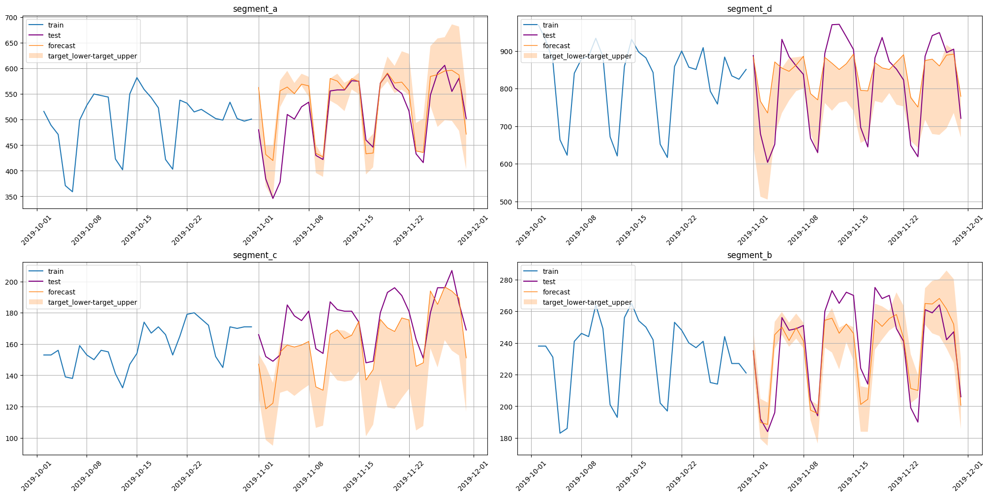
[22]:
plot_forecast(forecast, test_ts, train_ts, prediction_intervals=True, n_train_samples=30)
[23]:
coverage, width = interval_metrics(test_ts=test_ts, forecast=forecast)
[24]:
coverage
[24]:
{'segment_a': 0.8333333333333334,
 'segment_b': 0.9333333333333333,
 'segment_c': 0.8666666666666667,
 'segment_d': 0.9666666666666667}
[25]:
width
[25]:
{'segment_a': 108.50105291374686,
 'segment_b': 46.55147330372556,
 'segment_c': 72.3575509237814,
 'segment_d': 414.01584353697956}
ConformalPredictionIntervals#
Estimates conformal prediction intervals:
Compute matrix of absolute residuals \(r_{it} = |\hat y_{it} - y_{it}|\) using k-fold historical backtest, where \(i\) is fold index.
Estimate corresponding quantiles levels using the provided coverage (e.g. apply Bonferroni correction).
Estimate quantiles for each horizon step separately using computed absolute residuals and levels.
Note: this method estimates arbitrary interval bounds that tend to provide a given coverage rate. So this method ignores the quantiles parameter of the forecast method.
Coverage rate and correction option should be set at the method initialization step.
[26]:
from etna.experimental.prediction_intervals import ConformalPredictionIntervals
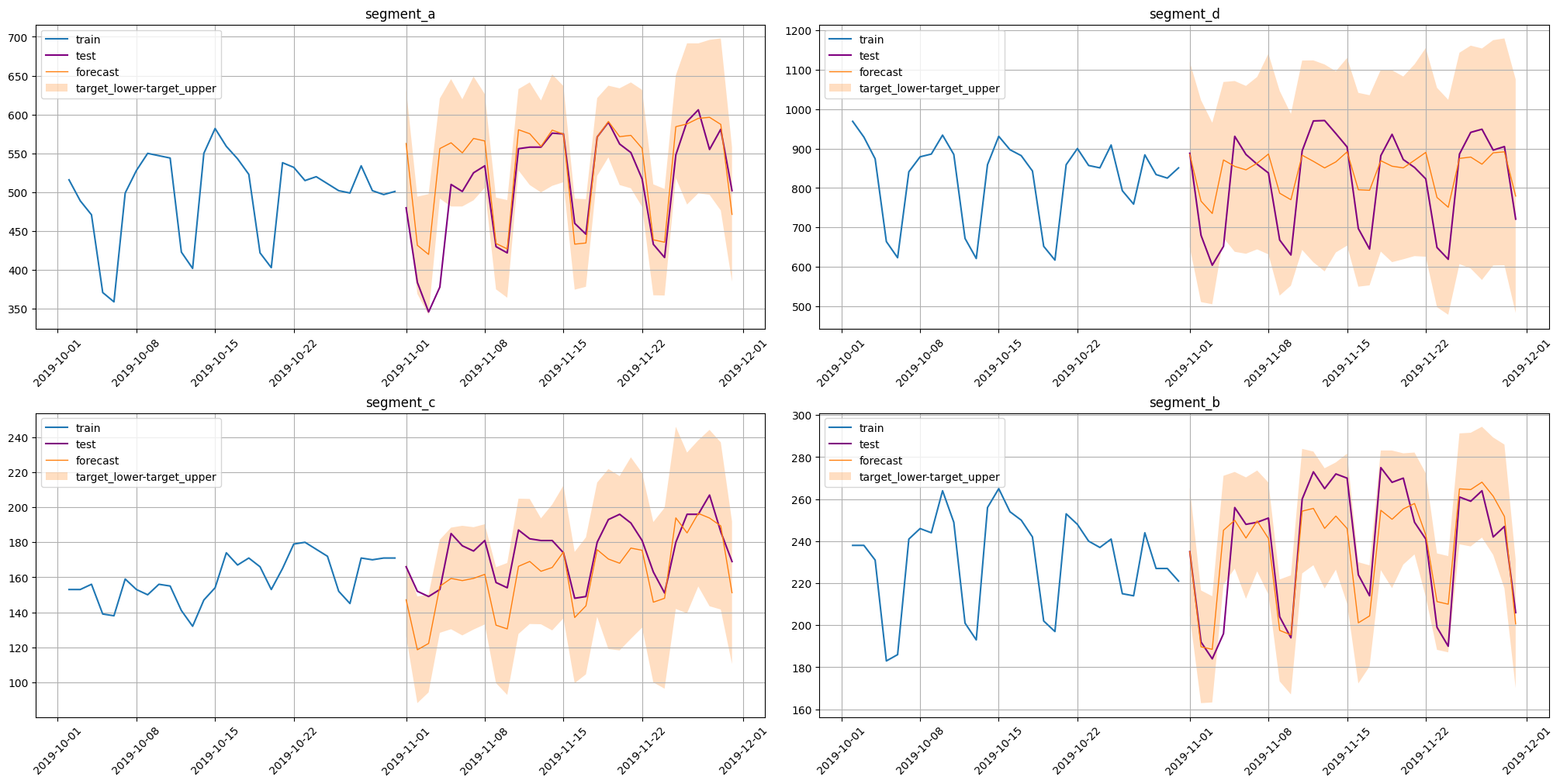
pipeline = ConformalPredictionIntervals(pipeline=pipeline, coverage=0.95, bonferroni_correction=True)
forecast = pipeline.forecast(prediction_interval=True, n_folds=40)
forecast
[Parallel(n_jobs=1)]: Using backend SequentialBackend with 1 concurrent workers.
[Parallel(n_jobs=1)]: Done   1 out of   1 | elapsed:    6.7s remaining:    0.0s
[Parallel(n_jobs=1)]: Done   2 out of   2 | elapsed:   13.9s remaining:    0.0s
[Parallel(n_jobs=1)]: Done   3 out of   3 | elapsed:   19.7s remaining:    0.0s
[Parallel(n_jobs=1)]: Done   4 out of   4 | elapsed:   25.1s remaining:    0.0s
[Parallel(n_jobs=1)]: Done   5 out of   5 | elapsed:   30.7s remaining:    0.0s
[Parallel(n_jobs=1)]: Done   6 out of   6 | elapsed:   39.9s remaining:    0.0s
[Parallel(n_jobs=1)]: Done   7 out of   7 | elapsed:   46.4s remaining:    0.0s
[Parallel(n_jobs=1)]: Done   8 out of   8 | elapsed:   52.3s remaining:    0.0s
[Parallel(n_jobs=1)]: Done   9 out of   9 | elapsed:   57.1s remaining:    0.0s
[Parallel(n_jobs=1)]: Done  10 out of  10 | elapsed:  1.0min remaining:    0.0s
[Parallel(n_jobs=1)]: Done  40 out of  40 | elapsed:  4.0min finished
[Parallel(n_jobs=1)]: Using backend SequentialBackend with 1 concurrent workers.
[Parallel(n_jobs=1)]: Done   1 out of   1 | elapsed:    0.2s remaining:    0.0s
[Parallel(n_jobs=1)]: Done   2 out of   2 | elapsed:    0.4s remaining:    0.0s
[Parallel(n_jobs=1)]: Done   3 out of   3 | elapsed:    0.6s remaining:    0.0s
[Parallel(n_jobs=1)]: Done   4 out of   4 | elapsed:    0.8s remaining:    0.0s
[Parallel(n_jobs=1)]: Done   5 out of   5 | elapsed:    1.0s remaining:    0.0s
[Parallel(n_jobs=1)]: Done   6 out of   6 | elapsed:    1.2s remaining:    0.0s
[Parallel(n_jobs=1)]: Done   7 out of   7 | elapsed:    1.4s remaining:    0.0s
[Parallel(n_jobs=1)]: Done   8 out of   8 | elapsed:    1.5s remaining:    0.0s
[Parallel(n_jobs=1)]: Done   9 out of   9 | elapsed:    1.7s remaining:    0.0s
[Parallel(n_jobs=1)]: Done  10 out of  10 | elapsed:    1.9s remaining:    0.0s
[Parallel(n_jobs=1)]: Done  40 out of  40 | elapsed:    6.1s finished
[Parallel(n_jobs=1)]: Using backend SequentialBackend with 1 concurrent workers.
[Parallel(n_jobs=1)]: Done   1 out of   1 | elapsed:    0.0s remaining:    0.0s
[Parallel(n_jobs=1)]: Done   2 out of   2 | elapsed:    0.0s remaining:    0.0s
[Parallel(n_jobs=1)]: Done   3 out of   3 | elapsed:    0.1s remaining:    0.0s
[Parallel(n_jobs=1)]: Done   4 out of   4 | elapsed:    0.1s remaining:    0.0s
[Parallel(n_jobs=1)]: Done   5 out of   5 | elapsed:    0.1s remaining:    0.0s
[Parallel(n_jobs=1)]: Done   6 out of   6 | elapsed:    0.1s remaining:    0.0s
[Parallel(n_jobs=1)]: Done   7 out of   7 | elapsed:    0.1s remaining:    0.0s
[Parallel(n_jobs=1)]: Done   8 out of   8 | elapsed:    0.2s remaining:    0.0s
[Parallel(n_jobs=1)]: Done   9 out of   9 | elapsed:    0.2s remaining:    0.0s
[Parallel(n_jobs=1)]: Done  10 out of  10 | elapsed:    0.2s remaining:    0.0s
[Parallel(n_jobs=1)]: Done  40 out of  40 | elapsed:    0.9s finished
[26]:
| segment | segment_a | ... | segment_d | ||||||||||||||||||
|---|---|---|---|---|---|---|---|---|---|---|---|---|---|---|---|---|---|---|---|---|---|
| feature | flag_day_number_in_month | flag_day_number_in_week | flag_is_weekend | flag_month_number_in_year | flag_week_number_in_month | flag_week_number_in_year | flag_year_number | lag_30 | lag_31 | lag_32 | ... | lag_44 | lag_45 | lag_46 | lag_47 | lag_48 | lag_49 | segment_code | target | target_lower | target_upper |
| timestamp | |||||||||||||||||||||
| 2019-11-01 | 1 | 4 | False | 11 | 1 | 44 | 2019 | 516.0 | 558.0 | 551.0 | ... | 860.0 | 859.0 | 833.0 | 592.0 | 616.0 | 824.0 | 3 | 884.890130 | 649.883469 | 1119.896790 |
| 2019-11-02 | 2 | 5 | True | 11 | 1 | 44 | 2019 | 489.0 | 516.0 | 558.0 | ... | 822.0 | 860.0 | 859.0 | 833.0 | 592.0 | 616.0 | 3 | 766.540795 | 510.541365 | 1022.540225 |
| 2019-11-03 | 3 | 6 | True | 11 | 1 | 44 | 2019 | 471.0 | 489.0 | 516.0 | ... | 908.0 | 822.0 | 860.0 | 859.0 | 833.0 | 592.0 | 3 | 735.275270 | 505.051234 | 965.499305 |
| 2019-11-04 | 4 | 0 | False | 11 | 2 | 45 | 2019 | 371.0 | 471.0 | 489.0 | ... | 648.0 | 908.0 | 822.0 | 860.0 | 859.0 | 833.0 | 3 | 871.086070 | 673.381908 | 1068.790232 |
| 2019-11-05 | 5 | 1 | False | 11 | 2 | 45 | 2019 | 359.0 | 371.0 | 471.0 | ... | 599.0 | 648.0 | 908.0 | 822.0 | 860.0 | 859.0 | 3 | 854.657442 | 638.063875 | 1071.251009 |
| 2019-11-06 | 6 | 2 | False | 11 | 2 | 45 | 2019 | 499.0 | 359.0 | 371.0 | ... | 821.0 | 599.0 | 648.0 | 908.0 | 822.0 | 860.0 | 3 | 845.998526 | 633.125621 | 1058.871431 |
| 2019-11-07 | 7 | 3 | False | 11 | 2 | 45 | 2019 | 528.0 | 499.0 | 359.0 | ... | 883.0 | 821.0 | 599.0 | 648.0 | 908.0 | 822.0 | 3 | 863.000343 | 644.282218 | 1081.718469 |
| 2019-11-08 | 8 | 4 | False | 11 | 2 | 45 | 2019 | 550.0 | 528.0 | 499.0 | ... | 923.0 | 883.0 | 821.0 | 599.0 | 648.0 | 908.0 | 3 | 886.018643 | 631.511196 | 1140.526090 |
| 2019-11-09 | 9 | 5 | True | 11 | 2 | 45 | 2019 | 547.0 | 550.0 | 528.0 | ... | 908.0 | 923.0 | 883.0 | 821.0 | 599.0 | 648.0 | 3 | 786.671129 | 526.983537 | 1046.358721 |
| 2019-11-10 | 10 | 6 | True | 11 | 2 | 45 | 2019 | 544.0 | 547.0 | 550.0 | ... | 874.0 | 908.0 | 923.0 | 883.0 | 821.0 | 599.0 | 3 | 770.142993 | 552.186714 | 988.099272 |
| 2019-11-11 | 11 | 0 | False | 11 | 3 | 46 | 2019 | 423.0 | 544.0 | 547.0 | ... | 712.0 | 874.0 | 908.0 | 923.0 | 883.0 | 821.0 | 3 | 883.026096 | 642.857515 | 1123.194676 |
| 2019-11-12 | 12 | 1 | False | 11 | 3 | 46 | 2019 | 402.0 | 423.0 | 544.0 | ... | 691.0 | 712.0 | 874.0 | 908.0 | 923.0 | 883.0 | 3 | 867.552488 | 611.475150 | 1123.629825 |
| 2019-11-13 | 13 | 2 | False | 11 | 3 | 46 | 2019 | 550.0 | 402.0 | 423.0 | ... | 980.0 | 691.0 | 712.0 | 874.0 | 908.0 | 923.0 | 3 | 850.850720 | 588.452817 | 1113.248622 |
| 2019-11-14 | 14 | 3 | False | 11 | 3 | 46 | 2019 | 582.0 | 550.0 | 402.0 | ... | 1037.0 | 980.0 | 691.0 | 712.0 | 874.0 | 908.0 | 3 | 866.155902 | 636.397113 | 1095.914691 |
| 2019-11-15 | 15 | 4 | False | 11 | 3 | 46 | 2019 | 559.0 | 582.0 | 550.0 | ... | 969.0 | 1037.0 | 980.0 | 691.0 | 712.0 | 874.0 | 3 | 891.686379 | 653.680738 | 1129.692021 |
| 2019-11-16 | 16 | 5 | True | 11 | 3 | 46 | 2019 | 543.0 | 559.0 | 582.0 | ... | 929.0 | 969.0 | 1037.0 | 980.0 | 691.0 | 712.0 | 3 | 795.462403 | 549.666908 | 1041.257899 |
| 2019-11-17 | 17 | 6 | True | 11 | 3 | 46 | 2019 | 523.0 | 543.0 | 559.0 | ... | 874.0 | 929.0 | 969.0 | 1037.0 | 980.0 | 691.0 | 3 | 794.104098 | 552.971103 | 1035.237093 |
| 2019-11-18 | 18 | 0 | False | 11 | 4 | 47 | 2019 | 422.0 | 523.0 | 543.0 | ... | 664.0 | 874.0 | 929.0 | 969.0 | 1037.0 | 980.0 | 3 | 869.079738 | 638.546838 | 1099.612638 |
| 2019-11-19 | 19 | 1 | False | 11 | 4 | 47 | 2019 | 403.0 | 422.0 | 523.0 | ... | 623.0 | 664.0 | 874.0 | 929.0 | 969.0 | 1037.0 | 3 | 855.177747 | 611.844429 | 1098.511065 |
| 2019-11-20 | 20 | 2 | False | 11 | 4 | 47 | 2019 | 538.0 | 403.0 | 422.0 | ... | 841.0 | 623.0 | 664.0 | 874.0 | 929.0 | 969.0 | 3 | 850.930059 | 619.085280 | 1082.774839 |
| 2019-11-21 | 21 | 3 | False | 11 | 4 | 47 | 2019 | 532.0 | 538.0 | 403.0 | ... | 879.0 | 841.0 | 623.0 | 664.0 | 874.0 | 929.0 | 3 | 870.278782 | 627.132036 | 1113.425529 |
| 2019-11-22 | 22 | 4 | False | 11 | 4 | 47 | 2019 | 515.0 | 532.0 | 538.0 | ... | 886.0 | 879.0 | 841.0 | 623.0 | 664.0 | 874.0 | 3 | 890.245006 | 625.590242 | 1154.899770 |
| 2019-11-23 | 23 | 5 | True | 11 | 4 | 47 | 2019 | 520.0 | 515.0 | 532.0 | ... | 934.0 | 886.0 | 879.0 | 841.0 | 623.0 | 664.0 | 3 | 775.886589 | 497.658120 | 1054.115058 |
| 2019-11-24 | 24 | 6 | True | 11 | 4 | 47 | 2019 | 511.0 | 520.0 | 515.0 | ... | 885.0 | 934.0 | 886.0 | 879.0 | 841.0 | 623.0 | 3 | 751.033775 | 478.400911 | 1023.666638 |
| 2019-11-25 | 25 | 0 | False | 11 | 5 | 48 | 2019 | 502.0 | 511.0 | 520.0 | ... | 672.0 | 885.0 | 934.0 | 886.0 | 879.0 | 841.0 | 3 | 874.921950 | 606.783185 | 1143.060715 |
| 2019-11-26 | 26 | 1 | False | 11 | 5 | 48 | 2019 | 499.0 | 502.0 | 511.0 | ... | 621.0 | 672.0 | 885.0 | 934.0 | 886.0 | 879.0 | 3 | 878.395149 | 595.791580 | 1160.998718 |
| 2019-11-27 | 27 | 2 | False | 11 | 5 | 48 | 2019 | 534.0 | 499.0 | 502.0 | ... | 859.0 | 621.0 | 672.0 | 885.0 | 934.0 | 886.0 | 3 | 860.259958 | 566.670708 | 1153.849209 |
| 2019-11-28 | 28 | 3 | False | 11 | 5 | 48 | 2019 | 502.0 | 534.0 | 499.0 | ... | 931.0 | 859.0 | 621.0 | 672.0 | 885.0 | 934.0 | 3 | 889.115142 | 603.341819 | 1174.888464 |
| 2019-11-29 | 29 | 4 | False | 11 | 5 | 48 | 2019 | 497.0 | 502.0 | 534.0 | ... | 897.0 | 931.0 | 859.0 | 621.0 | 672.0 | 885.0 | 3 | 891.706478 | 604.005315 | 1179.407642 |
| 2019-11-30 | 30 | 5 | True | 11 | 5 | 48 | 2019 | 501.0 | 497.0 | 502.0 | ... | 882.0 | 897.0 | 931.0 | 859.0 | 621.0 | 672.0 | 3 | 779.465792 | 483.160342 | 1075.771241 |
30 rows × 124 columns
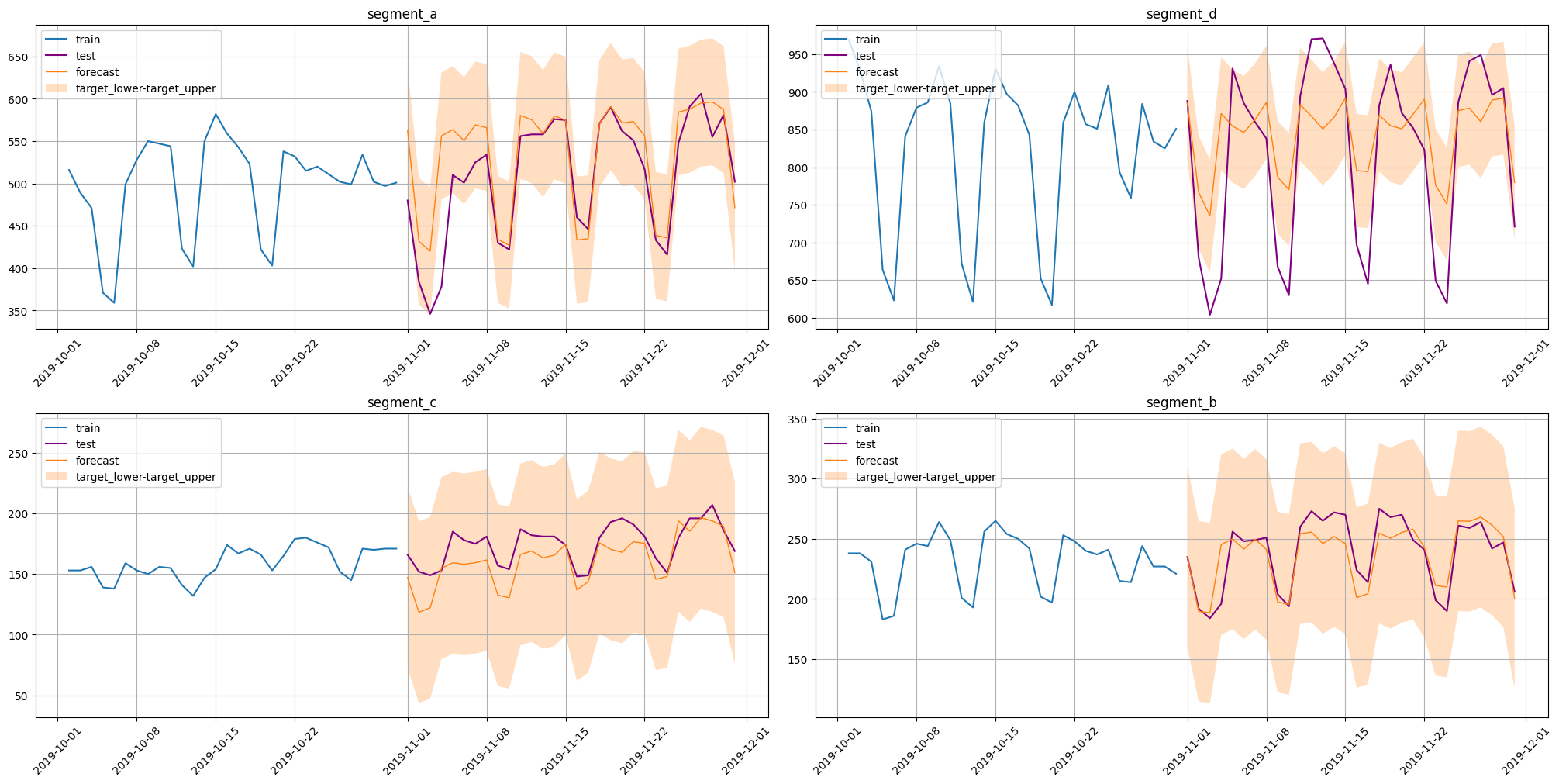
[27]:
plot_forecast(forecast, test_ts, train_ts, prediction_intervals=True, n_train_samples=30)
[28]:
coverage, width = interval_metrics(test_ts=test_ts, forecast=forecast)
[29]:
coverage
[29]:
{'segment_a': 0.9333333333333333,
 'segment_b': 0.9666666666666667,
 'segment_c': 0.9666666666666667,
 'segment_d': 0.9666666666666667}
[30]:
width
[30]:
{'segment_a': 141.19971750106404,
 'segment_b': 54.86083262147848,
 'segment_c': 77.48869154071357,
 'segment_d': 499.4061536460892}
EmpiricalPredictionIntervals#
Estimates prediction intervals via historical residuals:
Compute matrix of residuals \(r_{it} = |\hat y_{it} - y_{it}|\) using k-fold backtest, where \(i\) is fold index.
Estimate quantiles levels, that satisfy the provided coverage, for the corresponding residuals distributions.
Estimate quantiles for each timestamp using computed residuals and levels.
Note: this method estimates arbitrary interval bounds that tend to provide a given coverage rate. So this method ignores the quantiles parameter of the forecast method.
Coverage rate and correction option should be set at method initialization step.
[31]:
from etna.experimental.prediction_intervals import EmpiricalPredictionIntervals

pipeline = EmpiricalPredictionIntervals(pipeline=pipeline)

forecast = pipeline.forecast(prediction_interval=True, n_folds=40)

forecast
[Parallel(n_jobs=1)]: Using backend SequentialBackend with 1 concurrent workers.
[Parallel(n_jobs=1)]: Done   1 out of   1 | elapsed:    5.8s remaining:    0.0s
[Parallel(n_jobs=1)]: Done   2 out of   2 | elapsed:   11.2s remaining:    0.0s
[Parallel(n_jobs=1)]: Done   3 out of   3 | elapsed:   16.7s remaining:    0.0s
[Parallel(n_jobs=1)]: Done   4 out of   4 | elapsed:   22.7s remaining:    0.0s
[Parallel(n_jobs=1)]: Done   5 out of   5 | elapsed:   30.9s remaining:    0.0s
[Parallel(n_jobs=1)]: Done   6 out of   6 | elapsed:   36.1s remaining:    0.0s
[Parallel(n_jobs=1)]: Done   7 out of   7 | elapsed:   41.5s remaining:    0.0s
[Parallel(n_jobs=1)]: Done   8 out of   8 | elapsed:   47.5s remaining:    0.0s
[Parallel(n_jobs=1)]: Done   9 out of   9 | elapsed:   53.0s remaining:    0.0s
[Parallel(n_jobs=1)]: Done  10 out of  10 | elapsed:   58.9s remaining:    0.0s
[Parallel(n_jobs=1)]: Done  40 out of  40 | elapsed:  4.5min finished
[Parallel(n_jobs=1)]: Using backend SequentialBackend with 1 concurrent workers.
[Parallel(n_jobs=1)]: Done   1 out of   1 | elapsed:    0.2s remaining:    0.0s
[Parallel(n_jobs=1)]: Done   2 out of   2 | elapsed:    0.4s remaining:    0.0s
[Parallel(n_jobs=1)]: Done   3 out of   3 | elapsed:    0.6s remaining:    0.0s
[Parallel(n_jobs=1)]: Done   4 out of   4 | elapsed:    0.7s remaining:    0.0s
[Parallel(n_jobs=1)]: Done   5 out of   5 | elapsed:    0.9s remaining:    0.0s
[Parallel(n_jobs=1)]: Done   6 out of   6 | elapsed:    1.1s remaining:    0.0s
[Parallel(n_jobs=1)]: Done   7 out of   7 | elapsed:    1.2s remaining:    0.0s
[Parallel(n_jobs=1)]: Done   8 out of   8 | elapsed:    1.4s remaining:    0.0s
[Parallel(n_jobs=1)]: Done   9 out of   9 | elapsed:    1.5s remaining:    0.0s
[Parallel(n_jobs=1)]: Done  10 out of  10 | elapsed:    1.7s remaining:    0.0s
[Parallel(n_jobs=1)]: Done  40 out of  40 | elapsed:    6.1s finished
[Parallel(n_jobs=1)]: Using backend SequentialBackend with 1 concurrent workers.
[Parallel(n_jobs=1)]: Done   1 out of   1 | elapsed:    0.0s remaining:    0.0s
[Parallel(n_jobs=1)]: Done   2 out of   2 | elapsed:    0.1s remaining:    0.0s
[Parallel(n_jobs=1)]: Done   3 out of   3 | elapsed:    0.1s remaining:    0.0s
[Parallel(n_jobs=1)]: Done   4 out of   4 | elapsed:    0.1s remaining:    0.0s
[Parallel(n_jobs=1)]: Done   5 out of   5 | elapsed:    0.1s remaining:    0.0s
[Parallel(n_jobs=1)]: Done   6 out of   6 | elapsed:    0.2s remaining:    0.0s
[Parallel(n_jobs=1)]: Done   7 out of   7 | elapsed:    0.2s remaining:    0.0s
[Parallel(n_jobs=1)]: Done   8 out of   8 | elapsed:    0.2s remaining:    0.0s
[Parallel(n_jobs=1)]: Done   9 out of   9 | elapsed:    0.2s remaining:    0.0s
[Parallel(n_jobs=1)]: Done  10 out of  10 | elapsed:    0.3s remaining:    0.0s
[Parallel(n_jobs=1)]: Done  40 out of  40 | elapsed:    1.1s finished
[31]:
| segment | segment_a | ... | segment_d | ||||||||||||||||||
|---|---|---|---|---|---|---|---|---|---|---|---|---|---|---|---|---|---|---|---|---|---|
| feature | flag_day_number_in_month | flag_day_number_in_week | flag_is_weekend | flag_month_number_in_year | flag_week_number_in_month | flag_week_number_in_year | flag_year_number | lag_30 | lag_31 | lag_32 | ... | lag_44 | lag_45 | lag_46 | lag_47 | lag_48 | lag_49 | segment_code | target | target_lower | target_upper |
| timestamp | |||||||||||||||||||||
| 2019-11-01 | 1 | 4 | False | 11 | 1 | 44 | 2019 | 516.0 | 558.0 | 551.0 | ... | 860.0 | 859.0 | 833.0 | 592.0 | 616.0 | 824.0 | 3 | 884.890130 | 663.833307 | 912.762716 |
| 2019-11-02 | 2 | 5 | True | 11 | 1 | 44 | 2019 | 489.0 | 516.0 | 558.0 | ... | 822.0 | 860.0 | 859.0 | 833.0 | 592.0 | 616.0 | 3 | 766.540795 | 569.030264 | 801.586843 |
| 2019-11-03 | 3 | 6 | True | 11 | 1 | 44 | 2019 | 471.0 | 489.0 | 516.0 | ... | 908.0 | 822.0 | 860.0 | 859.0 | 833.0 | 592.0 | 3 | 735.275270 | 507.103746 | 778.679820 |
| 2019-11-04 | 4 | 0 | False | 11 | 2 | 45 | 2019 | 371.0 | 471.0 | 489.0 | ... | 648.0 | 908.0 | 822.0 | 860.0 | 859.0 | 833.0 | 3 | 871.086070 | 681.515744 | 901.930019 |
| 2019-11-05 | 5 | 1 | False | 11 | 2 | 45 | 2019 | 359.0 | 371.0 | 471.0 | ... | 599.0 | 648.0 | 908.0 | 822.0 | 860.0 | 859.0 | 3 | 854.657442 | 641.407846 | 866.047086 |
| 2019-11-06 | 6 | 2 | False | 11 | 2 | 45 | 2019 | 499.0 | 359.0 | 371.0 | ... | 821.0 | 599.0 | 648.0 | 908.0 | 822.0 | 860.0 | 3 | 845.998526 | 660.217161 | 867.762434 |
| 2019-11-07 | 7 | 3 | False | 11 | 2 | 45 | 2019 | 528.0 | 499.0 | 359.0 | ... | 883.0 | 821.0 | 599.0 | 648.0 | 908.0 | 822.0 | 3 | 863.000343 | 659.673561 | 882.054801 |
| 2019-11-08 | 8 | 4 | False | 11 | 2 | 45 | 2019 | 550.0 | 528.0 | 499.0 | ... | 923.0 | 883.0 | 821.0 | 599.0 | 648.0 | 908.0 | 3 | 886.018643 | 679.139431 | 886.018643 |
| 2019-11-09 | 9 | 5 | True | 11 | 2 | 45 | 2019 | 547.0 | 550.0 | 528.0 | ... | 908.0 | 923.0 | 883.0 | 821.0 | 599.0 | 648.0 | 3 | 786.671129 | 575.006386 | 786.671129 |
| 2019-11-10 | 10 | 6 | True | 11 | 2 | 45 | 2019 | 544.0 | 547.0 | 550.0 | ... | 874.0 | 908.0 | 923.0 | 883.0 | 821.0 | 599.0 | 3 | 770.142993 | 557.823008 | 770.142993 |
| 2019-11-11 | 11 | 0 | False | 11 | 3 | 46 | 2019 | 423.0 | 544.0 | 547.0 | ... | 712.0 | 874.0 | 908.0 | 923.0 | 883.0 | 821.0 | 3 | 883.026096 | 685.016228 | 883.026096 |
| 2019-11-12 | 12 | 1 | False | 11 | 3 | 46 | 2019 | 402.0 | 423.0 | 544.0 | ... | 691.0 | 712.0 | 874.0 | 908.0 | 923.0 | 883.0 | 3 | 867.552488 | 643.820651 | 867.552488 |
| 2019-11-13 | 13 | 2 | False | 11 | 3 | 46 | 2019 | 550.0 | 402.0 | 423.0 | ... | 980.0 | 691.0 | 712.0 | 874.0 | 908.0 | 923.0 | 3 | 850.850720 | 621.234961 | 850.850720 |
| 2019-11-14 | 14 | 3 | False | 11 | 3 | 46 | 2019 | 582.0 | 550.0 | 402.0 | ... | 1037.0 | 980.0 | 691.0 | 712.0 | 874.0 | 908.0 | 3 | 866.155902 | 659.104947 | 866.155902 |
| 2019-11-15 | 15 | 4 | False | 11 | 3 | 46 | 2019 | 559.0 | 582.0 | 550.0 | ... | 969.0 | 1037.0 | 980.0 | 691.0 | 712.0 | 874.0 | 3 | 891.686379 | 661.206654 | 891.686379 |
| 2019-11-16 | 16 | 5 | True | 11 | 3 | 46 | 2019 | 543.0 | 559.0 | 582.0 | ... | 929.0 | 969.0 | 1037.0 | 980.0 | 691.0 | 712.0 | 3 | 795.462403 | 567.609030 | 795.462403 |
| 2019-11-17 | 17 | 6 | True | 11 | 3 | 46 | 2019 | 523.0 | 543.0 | 559.0 | ... | 874.0 | 929.0 | 969.0 | 1037.0 | 980.0 | 691.0 | 3 | 794.104098 | 575.237147 | 794.104098 |
| 2019-11-18 | 18 | 0 | False | 11 | 4 | 47 | 2019 | 422.0 | 523.0 | 543.0 | ... | 664.0 | 874.0 | 929.0 | 969.0 | 1037.0 | 980.0 | 3 | 869.079738 | 672.336771 | 869.079738 |
| 2019-11-19 | 19 | 1 | False | 11 | 4 | 47 | 2019 | 403.0 | 422.0 | 523.0 | ... | 623.0 | 664.0 | 874.0 | 929.0 | 969.0 | 1037.0 | 3 | 855.177747 | 640.234380 | 855.177747 |
| 2019-11-20 | 20 | 2 | False | 11 | 4 | 47 | 2019 | 538.0 | 403.0 | 422.0 | ... | 841.0 | 623.0 | 664.0 | 874.0 | 929.0 | 969.0 | 3 | 850.930059 | 629.823414 | 850.930059 |
| 2019-11-21 | 21 | 3 | False | 11 | 4 | 47 | 2019 | 532.0 | 538.0 | 403.0 | ... | 879.0 | 841.0 | 623.0 | 664.0 | 874.0 | 929.0 | 3 | 870.278782 | 638.128801 | 870.278782 |
| 2019-11-22 | 22 | 4 | False | 11 | 4 | 47 | 2019 | 515.0 | 532.0 | 538.0 | ... | 886.0 | 879.0 | 841.0 | 623.0 | 664.0 | 874.0 | 3 | 890.245006 | 654.294956 | 890.245006 |
| 2019-11-23 | 23 | 5 | True | 11 | 4 | 47 | 2019 | 520.0 | 515.0 | 532.0 | ... | 934.0 | 886.0 | 879.0 | 841.0 | 623.0 | 664.0 | 3 | 775.886589 | 518.248701 | 777.189834 |
| 2019-11-24 | 24 | 6 | True | 11 | 4 | 47 | 2019 | 511.0 | 520.0 | 515.0 | ... | 885.0 | 934.0 | 886.0 | 879.0 | 841.0 | 623.0 | 3 | 751.033775 | 489.768310 | 751.033775 |
| 2019-11-25 | 25 | 0 | False | 11 | 5 | 48 | 2019 | 502.0 | 511.0 | 520.0 | ... | 672.0 | 885.0 | 934.0 | 886.0 | 879.0 | 841.0 | 3 | 874.921950 | 620.295448 | 874.921950 |
| 2019-11-26 | 26 | 1 | False | 11 | 5 | 48 | 2019 | 499.0 | 502.0 | 511.0 | ... | 621.0 | 672.0 | 885.0 | 934.0 | 886.0 | 879.0 | 3 | 878.395149 | 635.385892 | 878.395149 |
| 2019-11-27 | 27 | 2 | False | 11 | 5 | 48 | 2019 | 534.0 | 499.0 | 502.0 | ... | 859.0 | 621.0 | 672.0 | 885.0 | 934.0 | 886.0 | 3 | 860.259958 | 605.707920 | 860.259958 |
| 2019-11-28 | 28 | 3 | False | 11 | 5 | 48 | 2019 | 502.0 | 534.0 | 499.0 | ... | 931.0 | 859.0 | 621.0 | 672.0 | 885.0 | 934.0 | 3 | 889.115142 | 619.360181 | 889.115142 |
| 2019-11-29 | 29 | 4 | False | 11 | 5 | 48 | 2019 | 497.0 | 502.0 | 534.0 | ... | 897.0 | 931.0 | 859.0 | 621.0 | 672.0 | 885.0 | 3 | 891.706478 | 633.501917 | 891.706478 |
| 2019-11-30 | 30 | 5 | True | 11 | 5 | 48 | 2019 | 501.0 | 497.0 | 502.0 | ... | 882.0 | 897.0 | 931.0 | 859.0 | 621.0 | 672.0 | 3 | 779.465792 | 516.031185 | 779.465792 |
30 rows × 124 columns
[32]:
plot_forecast(forecast, test_ts, train_ts, prediction_intervals=True, n_train_samples=30)
[33]:
coverage, width = interval_metrics(test_ts=test_ts, forecast=forecast)
[34]:
coverage
[34]:
{'segment_a': 0.8666666666666667,
 'segment_b': 0.9333333333333333,
 'segment_c': 0.16666666666666666,
 'segment_d': 0.4666666666666667}
[35]:
width
[35]:
{'segment_a': 97.76013455528955,
 'segment_b': 40.370329153680345,
 'segment_c': 40.2553666590423,
 'segment_d': 231.97320117702435}
Prediction intervals for ensembles#
Pipeline ensembles could be passed to interval methods as well.
Consider a short usage example with VotingEnsemble.
[36]:
from etna.ensembles import VotingEnsemble

ensemble = VotingEnsemble(pipelines=[deepcopy(pipeline), deepcopy(pipeline)])
ensemble = NaiveVariancePredictionIntervals(pipeline=ensemble, stride=HORIZON)

forecast = pipeline.forecast(prediction_interval=True, n_folds=5)

forecast.prediction_intervals_names
[Parallel(n_jobs=1)]: Using backend SequentialBackend with 1 concurrent workers.
[Parallel(n_jobs=1)]: Done   1 out of   1 | elapsed:    7.8s remaining:    0.0s
[Parallel(n_jobs=1)]: Done   2 out of   2 | elapsed:   14.5s remaining:    0.0s
[Parallel(n_jobs=1)]: Done   3 out of   3 | elapsed:   21.2s remaining:    0.0s
[Parallel(n_jobs=1)]: Done   4 out of   4 | elapsed:   27.6s remaining:    0.0s
[Parallel(n_jobs=1)]: Done   5 out of   5 | elapsed:   35.0s remaining:    0.0s
[Parallel(n_jobs=1)]: Done   5 out of   5 | elapsed:   35.0s finished
[Parallel(n_jobs=1)]: Using backend SequentialBackend with 1 concurrent workers.
[Parallel(n_jobs=1)]: Done   1 out of   1 | elapsed:    0.2s remaining:    0.0s
[Parallel(n_jobs=1)]: Done   2 out of   2 | elapsed:    0.4s remaining:    0.0s
[Parallel(n_jobs=1)]: Done   3 out of   3 | elapsed:    0.6s remaining:    0.0s
[Parallel(n_jobs=1)]: Done   4 out of   4 | elapsed:    0.7s remaining:    0.0s
[Parallel(n_jobs=1)]: Done   5 out of   5 | elapsed:    0.9s remaining:    0.0s
[Parallel(n_jobs=1)]: Done   5 out of   5 | elapsed:    0.9s finished
[Parallel(n_jobs=1)]: Using backend SequentialBackend with 1 concurrent workers.
[Parallel(n_jobs=1)]: Done   1 out of   1 | elapsed:    0.0s remaining:    0.0s
[Parallel(n_jobs=1)]: Done   2 out of   2 | elapsed:    0.1s remaining:    0.0s
[Parallel(n_jobs=1)]: Done   3 out of   3 | elapsed:    0.1s remaining:    0.0s
[Parallel(n_jobs=1)]: Done   4 out of   4 | elapsed:    0.1s remaining:    0.0s
[Parallel(n_jobs=1)]: Done   5 out of   5 | elapsed:    0.1s remaining:    0.0s
[Parallel(n_jobs=1)]: Done   5 out of   5 | elapsed:    0.1s finished
[36]:
('target_lower', 'target_upper')
[37]:
plot_forecast(forecast, test_ts, train_ts, prediction_intervals=True, n_train_samples=30)
Custom prediction interval method#
There is a possibility in the library to extend the set of prediction intervals methods by implementing the desired algorithm. This section demonstrates how it can be done. Examples of interface and utilities usage are provided as well.
BasePredictionIntervals - base class for prediction intervals methods.
This class implements a wrapper interface for pipelines and ensembles that provides the ability to estimate prediction intervals. So it requires a pipeline instance to be provided to the __init__ method for proper initialization.
To add a particular method for pipelines, one must inherit from this class and provide an implementation for the abstract method _forecast_prediction_interval. This method should estimate and store prediction intervals for out-of-sample forecasts.
Limitations In-sample prediction is not supported by default and will raise a corresponding error while attempting to do so. This functionality could be implemented if needed by overriding the _predict method, which is responsible for building an in-sample point forecast and adding prediction intervals.
Non-parametric method#
The example below demonstrates how the interval method could be implemented.
Consider ConstantWidthInterval, which simply adds constant width to a point forecast. Here width is a hyperparameter that will be set on the method initialization step.
[38]:
from typing import Sequence

from etna.experimental.prediction_intervals import BasePredictionIntervals
from etna.pipeline import BasePipeline
[39]:
class ConstantWidthInterval(BasePredictionIntervals):
    def __init__(self, pipeline: BasePipeline, interval_width: float):
        assert interval_width > 0

        self.interval_width = interval_width
        super().__init__(pipeline=pipeline)

    def _forecast_prediction_interval(
        self, ts: TSDataset, predictions: TSDataset, quantiles: Sequence[float], n_folds: int
    ) -> TSDataset:
        predicted_target = predictions[..., "target"]

        lower_border = predicted_target - self.interval_width / 2
        upper_border = predicted_target + self.interval_width / 2

        upper_border.rename({"target": "target_upper"}, inplace=True, axis=1)
        lower_border.rename({"target": "target_lower"}, inplace=True, axis=1)

        predictions.add_prediction_intervals(prediction_intervals_df=pd.concat([lower_border, upper_border], axis=1))
        return predictions
[40]:
pipeline = ConstantWidthInterval(pipeline=pipeline, interval_width=150)

forecast = pipeline.forecast(prediction_interval=True, n_folds=40)

forecast
[40]:
| segment | segment_a | ... | segment_d | ||||||||||||||||||
|---|---|---|---|---|---|---|---|---|---|---|---|---|---|---|---|---|---|---|---|---|---|
| feature | flag_day_number_in_month | flag_day_number_in_week | flag_is_weekend | flag_month_number_in_year | flag_week_number_in_month | flag_week_number_in_year | flag_year_number | lag_30 | lag_31 | lag_32 | ... | lag_44 | lag_45 | lag_46 | lag_47 | lag_48 | lag_49 | segment_code | target | target_lower | target_upper |
| timestamp | |||||||||||||||||||||
| 2019-11-01 | 1 | 4 | False | 11 | 1 | 44 | 2019 | 516.0 | 558.0 | 551.0 | ... | 860.0 | 859.0 | 833.0 | 592.0 | 616.0 | 824.0 | 3 | 884.890130 | 809.890130 | 959.890130 |
| 2019-11-02 | 2 | 5 | True | 11 | 1 | 44 | 2019 | 489.0 | 516.0 | 558.0 | ... | 822.0 | 860.0 | 859.0 | 833.0 | 592.0 | 616.0 | 3 | 766.540795 | 691.540795 | 841.540795 |
| 2019-11-03 | 3 | 6 | True | 11 | 1 | 44 | 2019 | 471.0 | 489.0 | 516.0 | ... | 908.0 | 822.0 | 860.0 | 859.0 | 833.0 | 592.0 | 3 | 735.275270 | 660.275270 | 810.275270 |
| 2019-11-04 | 4 | 0 | False | 11 | 2 | 45 | 2019 | 371.0 | 471.0 | 489.0 | ... | 648.0 | 908.0 | 822.0 | 860.0 | 859.0 | 833.0 | 3 | 871.086070 | 796.086070 | 946.086070 |
| 2019-11-05 | 5 | 1 | False | 11 | 2 | 45 | 2019 | 359.0 | 371.0 | 471.0 | ... | 599.0 | 648.0 | 908.0 | 822.0 | 860.0 | 859.0 | 3 | 854.657442 | 779.657442 | 929.657442 |
| 2019-11-06 | 6 | 2 | False | 11 | 2 | 45 | 2019 | 499.0 | 359.0 | 371.0 | ... | 821.0 | 599.0 | 648.0 | 908.0 | 822.0 | 860.0 | 3 | 845.998526 | 770.998526 | 920.998526 |
| 2019-11-07 | 7 | 3 | False | 11 | 2 | 45 | 2019 | 528.0 | 499.0 | 359.0 | ... | 883.0 | 821.0 | 599.0 | 648.0 | 908.0 | 822.0 | 3 | 863.000343 | 788.000343 | 938.000343 |
| 2019-11-08 | 8 | 4 | False | 11 | 2 | 45 | 2019 | 550.0 | 528.0 | 499.0 | ... | 923.0 | 883.0 | 821.0 | 599.0 | 648.0 | 908.0 | 3 | 886.018643 | 811.018643 | 961.018643 |
| 2019-11-09 | 9 | 5 | True | 11 | 2 | 45 | 2019 | 547.0 | 550.0 | 528.0 | ... | 908.0 | 923.0 | 883.0 | 821.0 | 599.0 | 648.0 | 3 | 786.671129 | 711.671129 | 861.671129 |
| 2019-11-10 | 10 | 6 | True | 11 | 2 | 45 | 2019 | 544.0 | 547.0 | 550.0 | ... | 874.0 | 908.0 | 923.0 | 883.0 | 821.0 | 599.0 | 3 | 770.142993 | 695.142993 | 845.142993 |
| 2019-11-11 | 11 | 0 | False | 11 | 3 | 46 | 2019 | 423.0 | 544.0 | 547.0 | ... | 712.0 | 874.0 | 908.0 | 923.0 | 883.0 | 821.0 | 3 | 883.026096 | 808.026096 | 958.026096 |
| 2019-11-12 | 12 | 1 | False | 11 | 3 | 46 | 2019 | 402.0 | 423.0 | 544.0 | ... | 691.0 | 712.0 | 874.0 | 908.0 | 923.0 | 883.0 | 3 | 867.552488 | 792.552488 | 942.552488 |
| 2019-11-13 | 13 | 2 | False | 11 | 3 | 46 | 2019 | 550.0 | 402.0 | 423.0 | ... | 980.0 | 691.0 | 712.0 | 874.0 | 908.0 | 923.0 | 3 | 850.850720 | 775.850720 | 925.850720 |
| 2019-11-14 | 14 | 3 | False | 11 | 3 | 46 | 2019 | 582.0 | 550.0 | 402.0 | ... | 1037.0 | 980.0 | 691.0 | 712.0 | 874.0 | 908.0 | 3 | 866.155902 | 791.155902 | 941.155902 |
| 2019-11-15 | 15 | 4 | False | 11 | 3 | 46 | 2019 | 559.0 | 582.0 | 550.0 | ... | 969.0 | 1037.0 | 980.0 | 691.0 | 712.0 | 874.0 | 3 | 891.686379 | 816.686379 | 966.686379 |
| 2019-11-16 | 16 | 5 | True | 11 | 3 | 46 | 2019 | 543.0 | 559.0 | 582.0 | ... | 929.0 | 969.0 | 1037.0 | 980.0 | 691.0 | 712.0 | 3 | 795.462403 | 720.462403 | 870.462403 |
| 2019-11-17 | 17 | 6 | True | 11 | 3 | 46 | 2019 | 523.0 | 543.0 | 559.0 | ... | 874.0 | 929.0 | 969.0 | 1037.0 | 980.0 | 691.0 | 3 | 794.104098 | 719.104098 | 869.104098 |
| 2019-11-18 | 18 | 0 | False | 11 | 4 | 47 | 2019 | 422.0 | 523.0 | 543.0 | ... | 664.0 | 874.0 | 929.0 | 969.0 | 1037.0 | 980.0 | 3 | 869.079738 | 794.079738 | 944.079738 |
| 2019-11-19 | 19 | 1 | False | 11 | 4 | 47 | 2019 | 403.0 | 422.0 | 523.0 | ... | 623.0 | 664.0 | 874.0 | 929.0 | 969.0 | 1037.0 | 3 | 855.177747 | 780.177747 | 930.177747 |
| 2019-11-20 | 20 | 2 | False | 11 | 4 | 47 | 2019 | 538.0 | 403.0 | 422.0 | ... | 841.0 | 623.0 | 664.0 | 874.0 | 929.0 | 969.0 | 3 | 850.930059 | 775.930059 | 925.930059 |
| 2019-11-21 | 21 | 3 | False | 11 | 4 | 47 | 2019 | 532.0 | 538.0 | 403.0 | ... | 879.0 | 841.0 | 623.0 | 664.0 | 874.0 | 929.0 | 3 | 870.278782 | 795.278782 | 945.278782 |
| 2019-11-22 | 22 | 4 | False | 11 | 4 | 47 | 2019 | 515.0 | 532.0 | 538.0 | ... | 886.0 | 879.0 | 841.0 | 623.0 | 664.0 | 874.0 | 3 | 890.245006 | 815.245006 | 965.245006 |
| 2019-11-23 | 23 | 5 | True | 11 | 4 | 47 | 2019 | 520.0 | 515.0 | 532.0 | ... | 934.0 | 886.0 | 879.0 | 841.0 | 623.0 | 664.0 | 3 | 775.886589 | 700.886589 | 850.886589 |
| 2019-11-24 | 24 | 6 | True | 11 | 4 | 47 | 2019 | 511.0 | 520.0 | 515.0 | ... | 885.0 | 934.0 | 886.0 | 879.0 | 841.0 | 623.0 | 3 | 751.033775 | 676.033775 | 826.033775 |
| 2019-11-25 | 25 | 0 | False | 11 | 5 | 48 | 2019 | 502.0 | 511.0 | 520.0 | ... | 672.0 | 885.0 | 934.0 | 886.0 | 879.0 | 841.0 | 3 | 874.921950 | 799.921950 | 949.921950 |
| 2019-11-26 | 26 | 1 | False | 11 | 5 | 48 | 2019 | 499.0 | 502.0 | 511.0 | ... | 621.0 | 672.0 | 885.0 | 934.0 | 886.0 | 879.0 | 3 | 878.395149 | 803.395149 | 953.395149 |
| 2019-11-27 | 27 | 2 | False | 11 | 5 | 48 | 2019 | 534.0 | 499.0 | 502.0 | ... | 859.0 | 621.0 | 672.0 | 885.0 | 934.0 | 886.0 | 3 | 860.259958 | 785.259958 | 935.259958 |
| 2019-11-28 | 28 | 3 | False | 11 | 5 | 48 | 2019 | 502.0 | 534.0 | 499.0 | ... | 931.0 | 859.0 | 621.0 | 672.0 | 885.0 | 934.0 | 3 | 889.115142 | 814.115142 | 964.115142 |
| 2019-11-29 | 29 | 4 | False | 11 | 5 | 48 | 2019 | 497.0 | 502.0 | 534.0 | ... | 897.0 | 931.0 | 859.0 | 621.0 | 672.0 | 885.0 | 3 | 891.706478 | 816.706478 | 966.706478 |
| 2019-11-30 | 30 | 5 | True | 11 | 5 | 48 | 2019 | 501.0 | 497.0 | 502.0 | ... | 882.0 | 897.0 | 931.0 | 859.0 | 621.0 | 672.0 | 3 | 779.465792 | 704.465792 | 854.465792 |
30 rows × 124 columns
[41]:
plot_forecast(forecast, test_ts, train_ts, prediction_intervals=True, n_train_samples=30)
[42]:
coverage, width = interval_metrics(test_ts=test_ts, forecast=forecast)
[43]:
coverage
[43]:
{'segment_a': 0.9333333333333333,
 'segment_b': 1.0,
 'segment_c': 1.0,
 'segment_d': 0.5333333333333333}
[44]:
width
[44]:
{'segment_a': 150.0,
 'segment_b': 150.0,
 'segment_c': 150.0,
 'segment_d': 150.0}
Estimating historical residuals#
Some prediction intervals methods require doing historical forecasts. This could be done by using the pipeline’s get_historical_forecasts method. As BasePredictionIntervals wraps pipelines, this method is implemented here as well.
Consider the example MaxAbsResidInterval. This method estimates intervals based on the maximum absolute values of historical residuals for each segment. So we can break down this algorithm into the following steps:
Estimate historical forecasts by calling the
get_historical_forecastsmethod.For each
segmentestimate residuals, find the maximum absolute value and add to the point forecast.
[45]:
class MaxAbsResidInterval(BasePredictionIntervals):
    def __init__(self, pipeline: BasePipeline, coverage: float = 0.95, stride: int = 1):
        assert stride > 0
        assert 0 < coverage <= 1

        self.stride = stride
        self.coverage = coverage
        super().__init__(pipeline=pipeline)

    def _forecast_prediction_interval(
        self, ts: TSDataset, predictions: TSDataset, quantiles: Sequence[float], n_folds: int
    ) -> TSDataset:
        predicted_target = predictions[..., "target"]

        lower_border = predicted_target.copy()
        upper_border = predicted_target.copy()

        fold_forecast = self.get_historical_forecasts(ts=ts, n_folds=n_folds, stride=self.stride)

        for segment in ts.segments:
            residuals = (
                ts.loc[:, pd.IndexSlice[segment, "target"]] - fold_forecast.loc[:, pd.IndexSlice[segment, "target"]]
            )
            width = np.max(np.abs(residuals))

            lower_border.loc[:, pd.IndexSlice[segment, "target"]] -= self.coverage * width / 2
            upper_border.loc[:, pd.IndexSlice[segment, "target"]] += self.coverage * width / 2

        upper_border.rename({"target": "target_upper"}, inplace=True, axis=1)
        lower_border.rename({"target": "target_lower"}, inplace=True, axis=1)

        predictions.add_prediction_intervals(prediction_intervals_df=pd.concat([lower_border, upper_border], axis=1))
        return predictions
[46]:
pipeline = MaxAbsResidInterval(pipeline=pipeline)

forecast = pipeline.forecast(prediction_interval=True, n_folds=5)

forecast
[Parallel(n_jobs=1)]: Using backend SequentialBackend with 1 concurrent workers.
[Parallel(n_jobs=1)]: Done   1 out of   1 | elapsed:    7.5s remaining:    0.0s
[Parallel(n_jobs=1)]: Done   2 out of   2 | elapsed:   13.5s remaining:    0.0s
[Parallel(n_jobs=1)]: Done   3 out of   3 | elapsed:   19.7s remaining:    0.0s
[Parallel(n_jobs=1)]: Done   4 out of   4 | elapsed:   26.4s remaining:    0.0s
[Parallel(n_jobs=1)]: Done   5 out of   5 | elapsed:   32.3s remaining:    0.0s
[Parallel(n_jobs=1)]: Done   5 out of   5 | elapsed:   32.3s finished
[Parallel(n_jobs=1)]: Using backend SequentialBackend with 1 concurrent workers.
[Parallel(n_jobs=1)]: Done   1 out of   1 | elapsed:    0.1s remaining:    0.0s
[Parallel(n_jobs=1)]: Done   2 out of   2 | elapsed:    0.3s remaining:    0.0s
[Parallel(n_jobs=1)]: Done   3 out of   3 | elapsed:    0.7s remaining:    0.0s
[Parallel(n_jobs=1)]: Done   4 out of   4 | elapsed:    0.9s remaining:    0.0s
[Parallel(n_jobs=1)]: Done   5 out of   5 | elapsed:    1.2s remaining:    0.0s
[Parallel(n_jobs=1)]: Done   5 out of   5 | elapsed:    1.2s finished
[Parallel(n_jobs=1)]: Using backend SequentialBackend with 1 concurrent workers.
[Parallel(n_jobs=1)]: Done   1 out of   1 | elapsed:    0.0s remaining:    0.0s
[Parallel(n_jobs=1)]: Done   2 out of   2 | elapsed:    0.1s remaining:    0.0s
[Parallel(n_jobs=1)]: Done   3 out of   3 | elapsed:    0.1s remaining:    0.0s
[Parallel(n_jobs=1)]: Done   4 out of   4 | elapsed:    0.2s remaining:    0.0s
[Parallel(n_jobs=1)]: Done   5 out of   5 | elapsed:    0.2s remaining:    0.0s
[Parallel(n_jobs=1)]: Done   5 out of   5 | elapsed:    0.2s finished
[46]:
| segment | segment_a | ... | segment_d | ||||||||||||||||||
|---|---|---|---|---|---|---|---|---|---|---|---|---|---|---|---|---|---|---|---|---|---|
| feature | flag_day_number_in_month | flag_day_number_in_week | flag_is_weekend | flag_month_number_in_year | flag_week_number_in_month | flag_week_number_in_year | flag_year_number | lag_30 | lag_31 | lag_32 | ... | lag_44 | lag_45 | lag_46 | lag_47 | lag_48 | lag_49 | segment_code | target | target_lower | target_upper |
| timestamp | |||||||||||||||||||||
| 2019-11-01 | 1 | 4 | False | 11 | 1 | 44 | 2019 | 516.0 | 558.0 | 551.0 | ... | 860.0 | 859.0 | 833.0 | 592.0 | 616.0 | 824.0 | 3 | 884.890130 | 761.305956 | 1008.474304 |
| 2019-11-02 | 2 | 5 | True | 11 | 1 | 44 | 2019 | 489.0 | 516.0 | 558.0 | ... | 822.0 | 860.0 | 859.0 | 833.0 | 592.0 | 616.0 | 3 | 766.540795 | 642.956621 | 890.124969 |
| 2019-11-03 | 3 | 6 | True | 11 | 1 | 44 | 2019 | 471.0 | 489.0 | 516.0 | ... | 908.0 | 822.0 | 860.0 | 859.0 | 833.0 | 592.0 | 3 | 735.275270 | 611.691096 | 858.859443 |
| 2019-11-04 | 4 | 0 | False | 11 | 2 | 45 | 2019 | 371.0 | 471.0 | 489.0 | ... | 648.0 | 908.0 | 822.0 | 860.0 | 859.0 | 833.0 | 3 | 871.086070 | 747.501896 | 994.670244 |
| 2019-11-05 | 5 | 1 | False | 11 | 2 | 45 | 2019 | 359.0 | 371.0 | 471.0 | ... | 599.0 | 648.0 | 908.0 | 822.0 | 860.0 | 859.0 | 3 | 854.657442 | 731.073268 | 978.241616 |
| 2019-11-06 | 6 | 2 | False | 11 | 2 | 45 | 2019 | 499.0 | 359.0 | 371.0 | ... | 821.0 | 599.0 | 648.0 | 908.0 | 822.0 | 860.0 | 3 | 845.998526 | 722.414352 | 969.582700 |
| 2019-11-07 | 7 | 3 | False | 11 | 2 | 45 | 2019 | 528.0 | 499.0 | 359.0 | ... | 883.0 | 821.0 | 599.0 | 648.0 | 908.0 | 822.0 | 3 | 863.000343 | 739.416169 | 986.584517 |
| 2019-11-08 | 8 | 4 | False | 11 | 2 | 45 | 2019 | 550.0 | 528.0 | 499.0 | ... | 923.0 | 883.0 | 821.0 | 599.0 | 648.0 | 908.0 | 3 | 886.018643 | 762.434469 | 1009.602817 |
| 2019-11-09 | 9 | 5 | True | 11 | 2 | 45 | 2019 | 547.0 | 550.0 | 528.0 | ... | 908.0 | 923.0 | 883.0 | 821.0 | 599.0 | 648.0 | 3 | 786.671129 | 663.086955 | 910.255303 |
| 2019-11-10 | 10 | 6 | True | 11 | 2 | 45 | 2019 | 544.0 | 547.0 | 550.0 | ... | 874.0 | 908.0 | 923.0 | 883.0 | 821.0 | 599.0 | 3 | 770.142993 | 646.558819 | 893.727167 |
| 2019-11-11 | 11 | 0 | False | 11 | 3 | 46 | 2019 | 423.0 | 544.0 | 547.0 | ... | 712.0 | 874.0 | 908.0 | 923.0 | 883.0 | 821.0 | 3 | 883.026096 | 759.441922 | 1006.610270 |
| 2019-11-12 | 12 | 1 | False | 11 | 3 | 46 | 2019 | 402.0 | 423.0 | 544.0 | ... | 691.0 | 712.0 | 874.0 | 908.0 | 923.0 | 883.0 | 3 | 867.552488 | 743.968314 | 991.136661 |
| 2019-11-13 | 13 | 2 | False | 11 | 3 | 46 | 2019 | 550.0 | 402.0 | 423.0 | ... | 980.0 | 691.0 | 712.0 | 874.0 | 908.0 | 923.0 | 3 | 850.850720 | 727.266546 | 974.434894 |
| 2019-11-14 | 14 | 3 | False | 11 | 3 | 46 | 2019 | 582.0 | 550.0 | 402.0 | ... | 1037.0 | 980.0 | 691.0 | 712.0 | 874.0 | 908.0 | 3 | 866.155902 | 742.571728 | 989.740076 |
| 2019-11-15 | 15 | 4 | False | 11 | 3 | 46 | 2019 | 559.0 | 582.0 | 550.0 | ... | 969.0 | 1037.0 | 980.0 | 691.0 | 712.0 | 874.0 | 3 | 891.686379 | 768.102206 | 1015.270553 |
| 2019-11-16 | 16 | 5 | True | 11 | 3 | 46 | 2019 | 543.0 | 559.0 | 582.0 | ... | 929.0 | 969.0 | 1037.0 | 980.0 | 691.0 | 712.0 | 3 | 795.462403 | 671.878230 | 919.046577 |
| 2019-11-17 | 17 | 6 | True | 11 | 3 | 46 | 2019 | 523.0 | 543.0 | 559.0 | ... | 874.0 | 929.0 | 969.0 | 1037.0 | 980.0 | 691.0 | 3 | 794.104098 | 670.519924 | 917.688272 |
| 2019-11-18 | 18 | 0 | False | 11 | 4 | 47 | 2019 | 422.0 | 523.0 | 543.0 | ... | 664.0 | 874.0 | 929.0 | 969.0 | 1037.0 | 980.0 | 3 | 869.079738 | 745.495564 | 992.663912 |
| 2019-11-19 | 19 | 1 | False | 11 | 4 | 47 | 2019 | 403.0 | 422.0 | 523.0 | ... | 623.0 | 664.0 | 874.0 | 929.0 | 969.0 | 1037.0 | 3 | 855.177747 | 731.593573 | 978.761921 |
| 2019-11-20 | 20 | 2 | False | 11 | 4 | 47 | 2019 | 538.0 | 403.0 | 422.0 | ... | 841.0 | 623.0 | 664.0 | 874.0 | 929.0 | 969.0 | 3 | 850.930059 | 727.345885 | 974.514233 |
| 2019-11-21 | 21 | 3 | False | 11 | 4 | 47 | 2019 | 532.0 | 538.0 | 403.0 | ... | 879.0 | 841.0 | 623.0 | 664.0 | 874.0 | 929.0 | 3 | 870.278782 | 746.694608 | 993.862956 |
| 2019-11-22 | 22 | 4 | False | 11 | 4 | 47 | 2019 | 515.0 | 532.0 | 538.0 | ... | 886.0 | 879.0 | 841.0 | 623.0 | 664.0 | 874.0 | 3 | 890.245006 | 766.660832 | 1013.829180 |
| 2019-11-23 | 23 | 5 | True | 11 | 4 | 47 | 2019 | 520.0 | 515.0 | 532.0 | ... | 934.0 | 886.0 | 879.0 | 841.0 | 623.0 | 664.0 | 3 | 775.886589 | 652.302415 | 899.470763 |
| 2019-11-24 | 24 | 6 | True | 11 | 4 | 47 | 2019 | 511.0 | 520.0 | 515.0 | ... | 885.0 | 934.0 | 886.0 | 879.0 | 841.0 | 623.0 | 3 | 751.033775 | 627.449601 | 874.617949 |
| 2019-11-25 | 25 | 0 | False | 11 | 5 | 48 | 2019 | 502.0 | 511.0 | 520.0 | ... | 672.0 | 885.0 | 934.0 | 886.0 | 879.0 | 841.0 | 3 | 874.921950 | 751.337776 | 998.506124 |
| 2019-11-26 | 26 | 1 | False | 11 | 5 | 48 | 2019 | 499.0 | 502.0 | 511.0 | ... | 621.0 | 672.0 | 885.0 | 934.0 | 886.0 | 879.0 | 3 | 878.395149 | 754.810975 | 1001.979323 |
| 2019-11-27 | 27 | 2 | False | 11 | 5 | 48 | 2019 | 534.0 | 499.0 | 502.0 | ... | 859.0 | 621.0 | 672.0 | 885.0 | 934.0 | 886.0 | 3 | 860.259958 | 736.675784 | 983.844132 |
| 2019-11-28 | 28 | 3 | False | 11 | 5 | 48 | 2019 | 502.0 | 534.0 | 499.0 | ... | 931.0 | 859.0 | 621.0 | 672.0 | 885.0 | 934.0 | 3 | 889.115142 | 765.530968 | 1012.699316 |
| 2019-11-29 | 29 | 4 | False | 11 | 5 | 48 | 2019 | 497.0 | 502.0 | 534.0 | ... | 897.0 | 931.0 | 859.0 | 621.0 | 672.0 | 885.0 | 3 | 891.706478 | 768.122305 | 1015.290652 |
| 2019-11-30 | 30 | 5 | True | 11 | 5 | 48 | 2019 | 501.0 | 497.0 | 502.0 | ... | 882.0 | 897.0 | 931.0 | 859.0 | 621.0 | 672.0 | 3 | 779.465792 | 655.881618 | 903.049966 |
30 rows × 124 columns
[47]:
plot_forecast(forecast, test_ts, train_ts, prediction_intervals=True, n_train_samples=30)
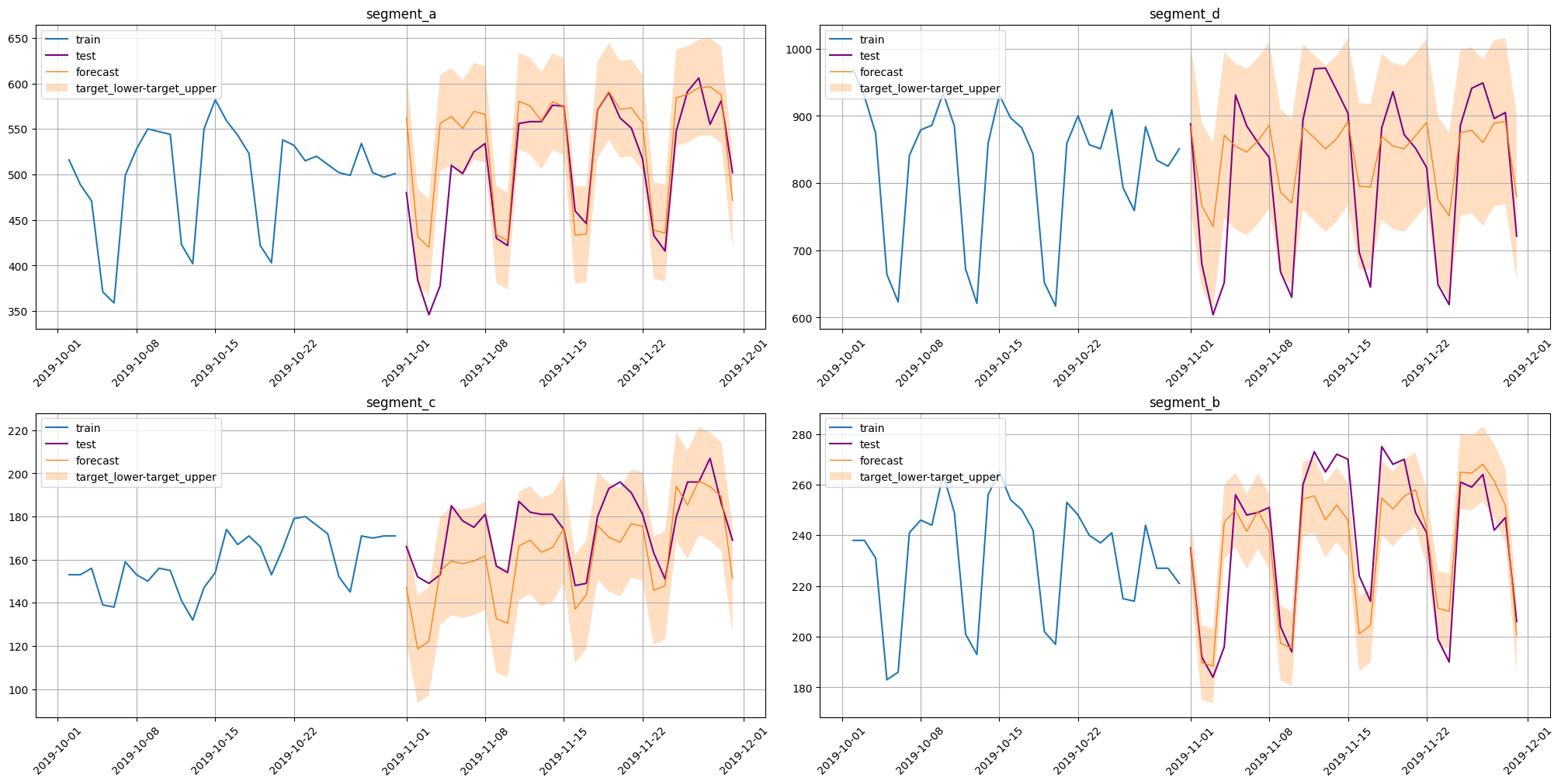
[48]:
coverage, width = interval_metrics(test_ts=test_ts, forecast=forecast)
[49]:
coverage
[49]:
{'segment_a': 0.8666666666666667,
 'segment_b': 0.6666666666666666,
 'segment_c': 0.8666666666666667,
 'segment_d': 0.8}
[50]:
width
[50]:
{'segment_a': 106.01589052275085,
 'segment_b': 29.46380276236236,
 'segment_c': 50.17717248209039,
 'segment_d': 247.16834782574568}
Obtaining historical residuals for prediction intervals estimation can be simplified by using the more efficient utility function residuals_matrices. This function accepts pipeline, data, parameters for backtest and computes residuals for each segment on every fold.
Note that residuals_matrices function returns a 3 dimensional array with axes sizes (num_folds, horizon, num_segments).
Here we use this function to optimize the proposed method. Consider OptimizedMaxAbsResidInterval.
[51]:
from etna.experimental.prediction_intervals.utils import residuals_matrices


class OptimizedMaxAbsResidInterval(BasePredictionIntervals):
    def __init__(self, pipeline: BasePipeline, coverage: float = 0.95, stride: int = 1):
        assert stride > 0
        assert 0 < coverage <= 1

        self.stride = stride
        self.coverage = coverage
        super().__init__(pipeline=pipeline)

    def _forecast_prediction_interval(
        self, ts: TSDataset, predictions: TSDataset, quantiles: Sequence[float], n_folds: int
    ) -> TSDataset:
        residuals = residuals_matrices(pipeline=self, ts=ts, n_folds=n_folds, stride=self.stride)

        predicted_target = predictions[..., "target"]

        width = np.max(np.abs(residuals), axis=(0, 1)).reshape(1, -1)

        lower_border = predicted_target - self.coverage * width / 2
        upper_border = predicted_target + self.coverage * width / 2

        upper_border.rename({"target": "target_upper"}, inplace=True, axis=1)
        lower_border.rename({"target": "target_lower"}, inplace=True, axis=1)

        predictions.add_prediction_intervals(prediction_intervals_df=pd.concat([lower_border, upper_border], axis=1))
        return predictions
[52]:
pipeline = OptimizedMaxAbsResidInterval(pipeline=pipeline)

forecast = pipeline.forecast(prediction_interval=True, n_folds=3)

forecast
[Parallel(n_jobs=1)]: Using backend SequentialBackend with 1 concurrent workers.
[Parallel(n_jobs=1)]: Done   1 out of   1 | elapsed:    6.6s remaining:    0.0s
[Parallel(n_jobs=1)]: Done   2 out of   2 | elapsed:   12.1s remaining:    0.0s
[Parallel(n_jobs=1)]: Done   3 out of   3 | elapsed:   17.8s remaining:    0.0s
[Parallel(n_jobs=1)]: Done   3 out of   3 | elapsed:   17.8s finished
[Parallel(n_jobs=1)]: Using backend SequentialBackend with 1 concurrent workers.
[Parallel(n_jobs=1)]: Done   1 out of   1 | elapsed:    0.1s remaining:    0.0s
[Parallel(n_jobs=1)]: Done   2 out of   2 | elapsed:    0.3s remaining:    0.0s
[Parallel(n_jobs=1)]: Done   3 out of   3 | elapsed:    0.4s remaining:    0.0s
[Parallel(n_jobs=1)]: Done   3 out of   3 | elapsed:    0.4s finished
[Parallel(n_jobs=1)]: Using backend SequentialBackend with 1 concurrent workers.
[Parallel(n_jobs=1)]: Done   1 out of   1 | elapsed:    0.0s remaining:    0.0s
[Parallel(n_jobs=1)]: Done   2 out of   2 | elapsed:    0.1s remaining:    0.0s
[Parallel(n_jobs=1)]: Done   3 out of   3 | elapsed:    0.1s remaining:    0.0s
[Parallel(n_jobs=1)]: Done   3 out of   3 | elapsed:    0.1s finished
[52]:
| segment | segment_a | ... | segment_d | ||||||||||||||||||
|---|---|---|---|---|---|---|---|---|---|---|---|---|---|---|---|---|---|---|---|---|---|
| feature | flag_day_number_in_month | flag_day_number_in_week | flag_is_weekend | flag_month_number_in_year | flag_week_number_in_month | flag_week_number_in_year | flag_year_number | lag_30 | lag_31 | lag_32 | ... | lag_44 | lag_45 | lag_46 | lag_47 | lag_48 | lag_49 | segment_code | target | target_lower | target_upper |
| timestamp | |||||||||||||||||||||
| 2019-11-01 | 1 | 4 | False | 11 | 1 | 44 | 2019 | 516.0 | 558.0 | 551.0 | ... | 860.0 | 859.0 | 833.0 | 592.0 | 616.0 | 824.0 | 3 | 884.890130 | 761.305956 | 1008.474304 |
| 2019-11-02 | 2 | 5 | True | 11 | 1 | 44 | 2019 | 489.0 | 516.0 | 558.0 | ... | 822.0 | 860.0 | 859.0 | 833.0 | 592.0 | 616.0 | 3 | 766.540795 | 642.956621 | 890.124969 |
| 2019-11-03 | 3 | 6 | True | 11 | 1 | 44 | 2019 | 471.0 | 489.0 | 516.0 | ... | 908.0 | 822.0 | 860.0 | 859.0 | 833.0 | 592.0 | 3 | 735.275270 | 611.691096 | 858.859443 |
| 2019-11-04 | 4 | 0 | False | 11 | 2 | 45 | 2019 | 371.0 | 471.0 | 489.0 | ... | 648.0 | 908.0 | 822.0 | 860.0 | 859.0 | 833.0 | 3 | 871.086070 | 747.501896 | 994.670244 |
| 2019-11-05 | 5 | 1 | False | 11 | 2 | 45 | 2019 | 359.0 | 371.0 | 471.0 | ... | 599.0 | 648.0 | 908.0 | 822.0 | 860.0 | 859.0 | 3 | 854.657442 | 731.073268 | 978.241616 |
| 2019-11-06 | 6 | 2 | False | 11 | 2 | 45 | 2019 | 499.0 | 359.0 | 371.0 | ... | 821.0 | 599.0 | 648.0 | 908.0 | 822.0 | 860.0 | 3 | 845.998526 | 722.414352 | 969.582700 |
| 2019-11-07 | 7 | 3 | False | 11 | 2 | 45 | 2019 | 528.0 | 499.0 | 359.0 | ... | 883.0 | 821.0 | 599.0 | 648.0 | 908.0 | 822.0 | 3 | 863.000343 | 739.416169 | 986.584517 |
| 2019-11-08 | 8 | 4 | False | 11 | 2 | 45 | 2019 | 550.0 | 528.0 | 499.0 | ... | 923.0 | 883.0 | 821.0 | 599.0 | 648.0 | 908.0 | 3 | 886.018643 | 762.434469 | 1009.602817 |
| 2019-11-09 | 9 | 5 | True | 11 | 2 | 45 | 2019 | 547.0 | 550.0 | 528.0 | ... | 908.0 | 923.0 | 883.0 | 821.0 | 599.0 | 648.0 | 3 | 786.671129 | 663.086955 | 910.255303 |
| 2019-11-10 | 10 | 6 | True | 11 | 2 | 45 | 2019 | 544.0 | 547.0 | 550.0 | ... | 874.0 | 908.0 | 923.0 | 883.0 | 821.0 | 599.0 | 3 | 770.142993 | 646.558819 | 893.727167 |
| 2019-11-11 | 11 | 0 | False | 11 | 3 | 46 | 2019 | 423.0 | 544.0 | 547.0 | ... | 712.0 | 874.0 | 908.0 | 923.0 | 883.0 | 821.0 | 3 | 883.026096 | 759.441922 | 1006.610270 |
| 2019-11-12 | 12 | 1 | False | 11 | 3 | 46 | 2019 | 402.0 | 423.0 | 544.0 | ... | 691.0 | 712.0 | 874.0 | 908.0 | 923.0 | 883.0 | 3 | 867.552488 | 743.968314 | 991.136661 |
| 2019-11-13 | 13 | 2 | False | 11 | 3 | 46 | 2019 | 550.0 | 402.0 | 423.0 | ... | 980.0 | 691.0 | 712.0 | 874.0 | 908.0 | 923.0 | 3 | 850.850720 | 727.266546 | 974.434894 |
| 2019-11-14 | 14 | 3 | False | 11 | 3 | 46 | 2019 | 582.0 | 550.0 | 402.0 | ... | 1037.0 | 980.0 | 691.0 | 712.0 | 874.0 | 908.0 | 3 | 866.155902 | 742.571728 | 989.740076 |
| 2019-11-15 | 15 | 4 | False | 11 | 3 | 46 | 2019 | 559.0 | 582.0 | 550.0 | ... | 969.0 | 1037.0 | 980.0 | 691.0 | 712.0 | 874.0 | 3 | 891.686379 | 768.102206 | 1015.270553 |
| 2019-11-16 | 16 | 5 | True | 11 | 3 | 46 | 2019 | 543.0 | 559.0 | 582.0 | ... | 929.0 | 969.0 | 1037.0 | 980.0 | 691.0 | 712.0 | 3 | 795.462403 | 671.878230 | 919.046577 |
| 2019-11-17 | 17 | 6 | True | 11 | 3 | 46 | 2019 | 523.0 | 543.0 | 559.0 | ... | 874.0 | 929.0 | 969.0 | 1037.0 | 980.0 | 691.0 | 3 | 794.104098 | 670.519924 | 917.688272 |
| 2019-11-18 | 18 | 0 | False | 11 | 4 | 47 | 2019 | 422.0 | 523.0 | 543.0 | ... | 664.0 | 874.0 | 929.0 | 969.0 | 1037.0 | 980.0 | 3 | 869.079738 | 745.495564 | 992.663912 |
| 2019-11-19 | 19 | 1 | False | 11 | 4 | 47 | 2019 | 403.0 | 422.0 | 523.0 | ... | 623.0 | 664.0 | 874.0 | 929.0 | 969.0 | 1037.0 | 3 | 855.177747 | 731.593573 | 978.761921 |
| 2019-11-20 | 20 | 2 | False | 11 | 4 | 47 | 2019 | 538.0 | 403.0 | 422.0 | ... | 841.0 | 623.0 | 664.0 | 874.0 | 929.0 | 969.0 | 3 | 850.930059 | 727.345885 | 974.514233 |
| 2019-11-21 | 21 | 3 | False | 11 | 4 | 47 | 2019 | 532.0 | 538.0 | 403.0 | ... | 879.0 | 841.0 | 623.0 | 664.0 | 874.0 | 929.0 | 3 | 870.278782 | 746.694608 | 993.862956 |
| 2019-11-22 | 22 | 4 | False | 11 | 4 | 47 | 2019 | 515.0 | 532.0 | 538.0 | ... | 886.0 | 879.0 | 841.0 | 623.0 | 664.0 | 874.0 | 3 | 890.245006 | 766.660832 | 1013.829180 |
| 2019-11-23 | 23 | 5 | True | 11 | 4 | 47 | 2019 | 520.0 | 515.0 | 532.0 | ... | 934.0 | 886.0 | 879.0 | 841.0 | 623.0 | 664.0 | 3 | 775.886589 | 652.302415 | 899.470763 |
| 2019-11-24 | 24 | 6 | True | 11 | 4 | 47 | 2019 | 511.0 | 520.0 | 515.0 | ... | 885.0 | 934.0 | 886.0 | 879.0 | 841.0 | 623.0 | 3 | 751.033775 | 627.449601 | 874.617949 |
| 2019-11-25 | 25 | 0 | False | 11 | 5 | 48 | 2019 | 502.0 | 511.0 | 520.0 | ... | 672.0 | 885.0 | 934.0 | 886.0 | 879.0 | 841.0 | 3 | 874.921950 | 751.337776 | 998.506124 |
| 2019-11-26 | 26 | 1 | False | 11 | 5 | 48 | 2019 | 499.0 | 502.0 | 511.0 | ... | 621.0 | 672.0 | 885.0 | 934.0 | 886.0 | 879.0 | 3 | 878.395149 | 754.810975 | 1001.979323 |
| 2019-11-27 | 27 | 2 | False | 11 | 5 | 48 | 2019 | 534.0 | 499.0 | 502.0 | ... | 859.0 | 621.0 | 672.0 | 885.0 | 934.0 | 886.0 | 3 | 860.259958 | 736.675784 | 983.844132 |
| 2019-11-28 | 28 | 3 | False | 11 | 5 | 48 | 2019 | 502.0 | 534.0 | 499.0 | ... | 931.0 | 859.0 | 621.0 | 672.0 | 885.0 | 934.0 | 3 | 889.115142 | 765.530968 | 1012.699316 |
| 2019-11-29 | 29 | 4 | False | 11 | 5 | 48 | 2019 | 497.0 | 502.0 | 534.0 | ... | 897.0 | 931.0 | 859.0 | 621.0 | 672.0 | 885.0 | 3 | 891.706478 | 768.122305 | 1015.290652 |
| 2019-11-30 | 30 | 5 | True | 11 | 5 | 48 | 2019 | 501.0 | 497.0 | 502.0 | ... | 882.0 | 897.0 | 931.0 | 859.0 | 621.0 | 672.0 | 3 | 779.465792 | 655.881618 | 903.049966 |
30 rows × 124 columns
[53]:
plot_forecast(forecast, test_ts, train_ts, prediction_intervals=True, n_train_samples=30)
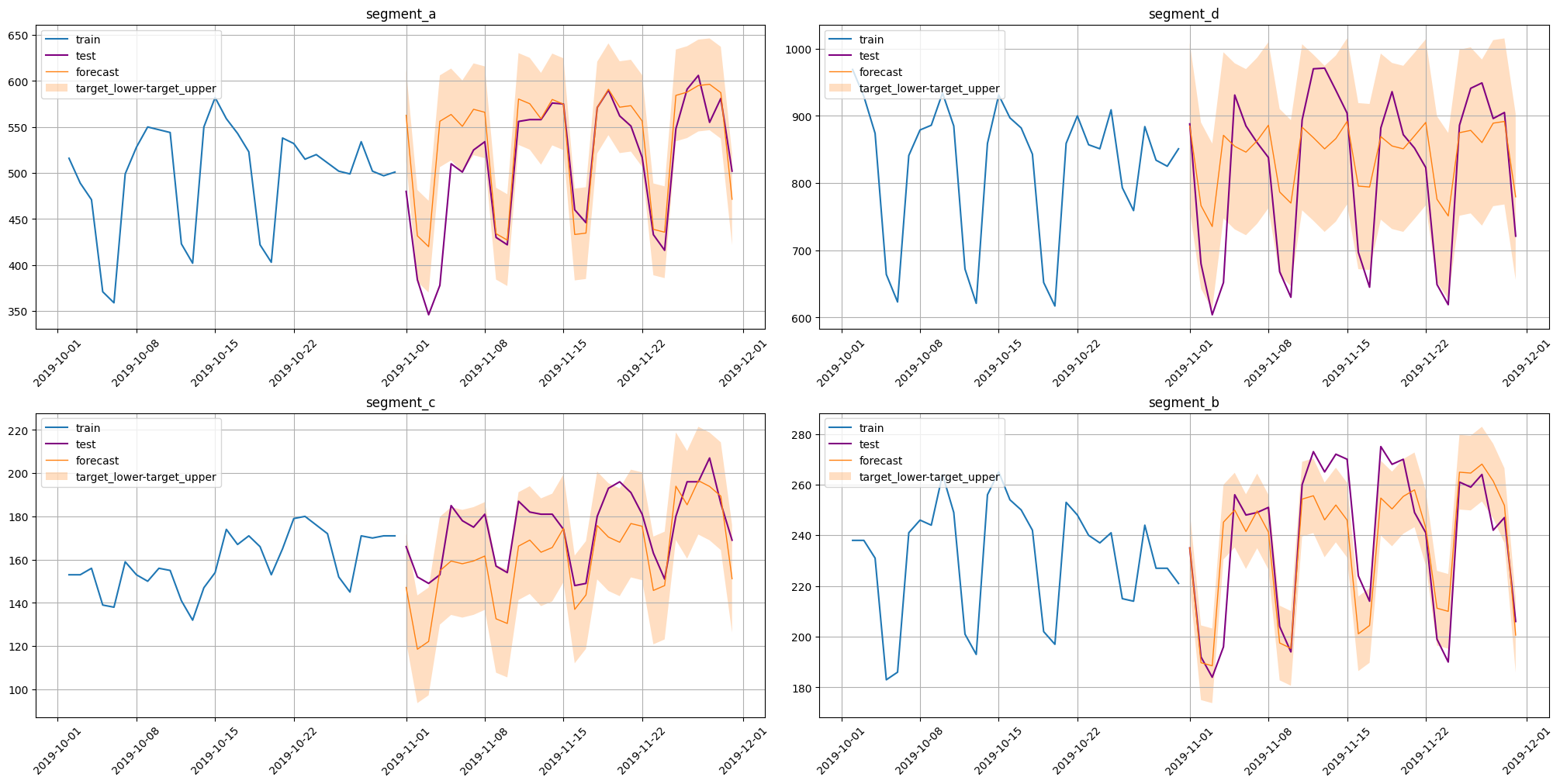
[54]:
coverage, width = interval_metrics(test_ts=test_ts, forecast=forecast)
[55]:
coverage
[55]:
{'segment_a': 0.8666666666666667,
 'segment_b': 0.6666666666666666,
 'segment_c': 0.8666666666666667,
 'segment_d': 0.8}
[56]:
width
[56]:
{'segment_a': 99.74407563536734,
 'segment_b': 29.46380276236236,
 'segment_c': 49.833980779974766,
 'segment_d': 247.16834782574568}