View Jupyter notebook on the GitHub.
Working with misaligned data#
![]()
This notebook contains the examples of working with misaligned data.
Table of contents
Loading data
Preparing data
Using ``TSDataset.create_from_misaligned` <#section_2_1>`__
Using ``infer_alignment` <#section_2_2>`__
Using ``apply_alignment` <#section_2_3>`__
Using ``make_timestamp_df_from_alignment` <#section_2_4>`__
Examples with regular data
Forecasting with ``CatBoostMultiSegmentModel` <#section_3_1>`__
Utilizing old data with ``CatBoostMultiSegmentModel` <#section_3_1>`__
Forecasting with ``ProphetModel` <#section_3_3>`__
Working with irregular data
[1]:
!pip install "etna[prophet]" -q
[2]:
import warnings

warnings.filterwarnings("ignore")
[3]:
import numpy as np
import pandas as pd

from etna.analysis import plot_backtest
from etna.datasets import TSDataset
from etna.metrics import SMAPE
from etna.models import CatBoostMultiSegmentModel
from etna.models import ProphetModel
from etna.pipeline import Pipeline
from etna.transforms import DateFlagsTransform
from etna.transforms import FourierTransform
from etna.transforms import HolidayTransform
from etna.transforms import LagTransform
from etna.transforms import LinearTrendTransform
from etna.transforms import LogTransform
from etna.transforms import MeanTransform
from etna.transforms import SegmentEncoderTransform
[4]:
HORIZON = 14
1. Loading data#
Let’s start by loading data with multiple segments.
[5]:
df = pd.read_csv("data/example_dataset.csv", parse_dates=["timestamp"])
df.head()
[5]:
| timestamp | segment | target | |
|---|---|---|---|
| 0 | 2019-01-01 | segment_a | 170 |
| 1 | 2019-01-02 | segment_a | 243 |
| 2 | 2019-01-03 | segment_a | 267 |
| 3 | 2019-01-04 | segment_a | 287 |
| 4 | 2019-01-05 | segment_a | 279 |
[6]:
ts = TSDataset(df, freq="D")
ts.plot()

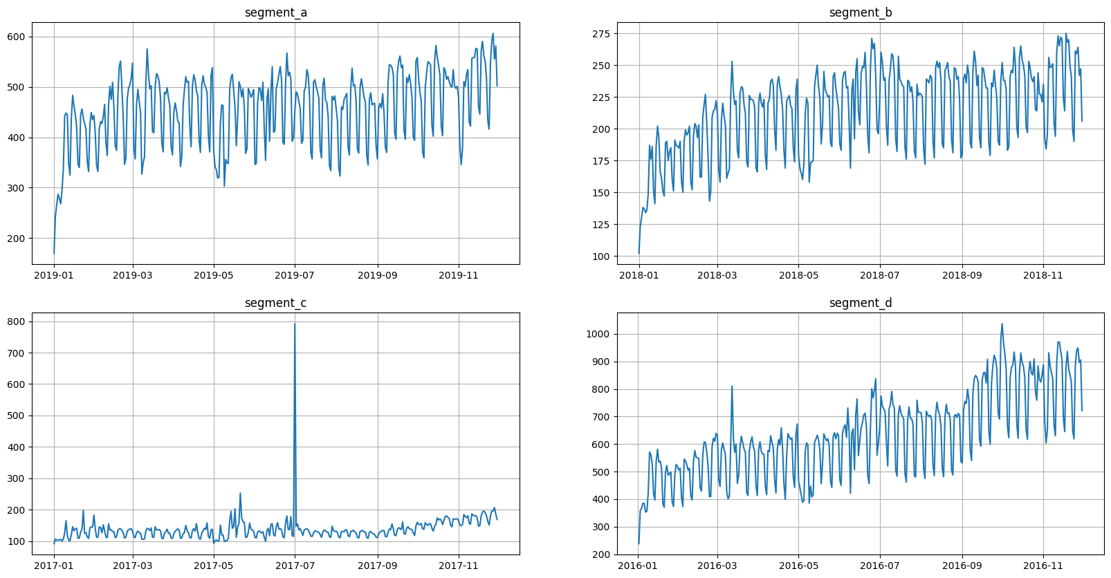
This data is aligned, but we need a misaligned data to make a demonstration. So, let’s shift the segments.
[7]:
df.loc[df["segment"] == "segment_b", "timestamp"] -= pd.Timedelta("365D")
df.loc[df["segment"] == "segment_c", "timestamp"] -= pd.Timedelta("730D")
df.loc[df["segment"] == "segment_d", "timestamp"] -= pd.Timedelta("1095D")
Now data is misaligned.
[8]:
ts_ma = TSDataset(df=df, freq="D")
ts_ma.plot()
2. Preparing data#
Our library by design works only with aligned data, so in order to support handling misaligned data we introduced the support of integer timestamp.
The idea is simple: if you have misaligned data you should create an integer timestamp that aligns times series with each other and then pass original timestamp as exogenous feature. In order to do all of this we added special utilities.
2.1 Using TSDataset.create_from_misaligned#
The most simple way to prepare data is to use a special constructor for TSDataset: TSDataset.create_from_misaligned.
Let’s try it out
[9]:
ts = TSDataset.create_from_misaligned(df=df, freq="D", future_steps=HORIZON)
ts.plot()

As we can see, now our time series are aligned by integer timestamp. There are few points to note: - Parameter df is expected to be in a long format. - The alignment is determined by the last timestamp for each segment. Last timestamp is taken without checking is target value missing or not.
Let’s look at ts to check the presence of original timestamp:
[10]:
ts.to_pandas()
[10]:
| segment | segment_a | segment_b | segment_c | segment_d | ||||
|---|---|---|---|---|---|---|---|---|
| feature | external_timestamp | target | external_timestamp | target | external_timestamp | target | external_timestamp | target |
| timestamp | ||||||||
| -333 | 2019-01-01 | 170.0 | 2018-01-01 | 102.0 | 2017-01-01 | 92.0 | 2016-01-02 | 238.0 |
| -332 | 2019-01-02 | 243.0 | 2018-01-02 | 123.0 | 2017-01-02 | 107.0 | 2016-01-03 | 358.0 |
| -331 | 2019-01-03 | 267.0 | 2018-01-03 | 130.0 | 2017-01-03 | 103.0 | 2016-01-04 | 366.0 |
| -330 | 2019-01-04 | 287.0 | 2018-01-04 | 138.0 | 2017-01-04 | 103.0 | 2016-01-05 | 385.0 |
| -329 | 2019-01-05 | 279.0 | 2018-01-05 | 137.0 | 2017-01-05 | 104.0 | 2016-01-06 | 384.0 |
| ... | ... | ... | ... | ... | ... | ... | ... | ... |
| -4 | 2019-11-26 | 591.0 | 2018-11-26 | 259.0 | 2017-11-26 | 196.0 | 2016-11-26 | 941.0 |
| -3 | 2019-11-27 | 606.0 | 2018-11-27 | 264.0 | 2017-11-27 | 196.0 | 2016-11-27 | 949.0 |
| -2 | 2019-11-28 | 555.0 | 2018-11-28 | 242.0 | 2017-11-28 | 207.0 | 2016-11-28 | 896.0 |
| -1 | 2019-11-29 | 581.0 | 2018-11-29 | 247.0 | 2017-11-29 | 186.0 | 2016-11-29 | 905.0 |
| 0 | 2019-11-30 | 502.0 | 2018-11-30 | 206.0 | 2017-11-30 | 169.0 | 2016-11-30 | 721.0 |
334 rows × 8 columns
The column with original timestamp is named external_timestamp, you could change the name by using a parameter named original_timestamp_name of TSDataset.create_from_misaligned.
The feature external_timestamp is a regressor and it is extended into the future by future_steps steps.
2.2 Using infer_alignment#
In addition to using TSDataset.create_from_misaligned we could also use a more specific utilities and repeat the creation of ts from misaligned data.
First, we should infer the alignment used in our data. For this we should use etna.datasets.infer_alignment.
[11]:
from etna.datasets import infer_alignment

alignment = infer_alignment(df)
alignment
[11]:
{'segment_a': Timestamp('2019-11-30 00:00:00'),
 'segment_b': Timestamp('2018-11-30 00:00:00'),
 'segment_c': Timestamp('2017-11-30 00:00:00'),
 'segment_d': Timestamp('2016-11-30 00:00:00')}
As we can see, the last timestamp is taken for each segment. These timestamps will have the same integer timestamp after creation of TSDataset.
2.3 Using apply_alignment#
The next step is to create our integer timestamp by using etna.datasets.apply_alignment.
[12]:
from etna.datasets import apply_alignment

df_aligned = apply_alignment(df=df, alignment=alignment, original_timestamp_name="external_timestamp")
df_aligned.head()
[12]:
| external_timestamp | segment | target | timestamp | |
|---|---|---|---|---|
| 0 | 2019-01-01 | segment_a | 170 | -333 |
| 1 | 2019-01-02 | segment_a | 243 | -332 |
| 2 | 2019-01-03 | segment_a | 267 | -331 |
| 3 | 2019-01-04 | segment_a | 287 | -330 |
| 4 | 2019-01-05 | segment_a | 279 | -329 |
As we can see, the original timestamp is saved under external_timestamp name. We don’t really need it, because we want it to be extended into the future.
[13]:
df_aligned = apply_alignment(df=df, alignment=alignment)
df_aligned.head()
[13]:
| timestamp | segment | target | |
|---|---|---|---|
| 0 | -333 | segment_a | 170 |
| 1 | -332 | segment_a | 243 |
| 2 | -331 | segment_a | 267 |
| 3 | -330 | segment_a | 287 |
| 4 | -329 | segment_a | 279 |
2.4 Using make_timestamp_df_from_alignment#
In order to make external_timestamp that extends into the future we are going to use etna.datasets.make_timestamp_df_from_alignment.
[14]:
from etna.datasets import make_timestamp_df_from_alignment

start_idx = df_aligned["timestamp"].min()
end_idx = df_aligned["timestamp"].max() + HORIZON
df_exog = make_timestamp_df_from_alignment(alignment=alignment, start=start_idx, end=end_idx, freq="D")
df_exog.head()
[14]:
| segment | timestamp | external_timestamp | |
|---|---|---|---|
| 0 | segment_a | -333 | 2019-01-01 |
| 1 | segment_a | -332 | 2019-01-02 |
| 2 | segment_a | -331 | 2019-01-03 |
| 3 | segment_a | -330 | 2019-01-04 |
| 4 | segment_a | -329 | 2019-01-05 |
As you might already guessed parameters start and end determines on which set of integer timestamps the datetime timestamp will be generated.
The only thing that remains is to create TSDataset. We should set freq=None, because now we are using integer timestamp.
[15]:
ts = TSDataset(df=df_aligned, df_exog=df_exog, freq=None, known_future="all")
ts.plot()

As we can see, the result is the same.
3. Examples with regular data#
3.1 Forecasting with CatBoostMultiSegmentModel#
Let’s see how to forecast misaligned data using CatBoostMultiSegmentModel. This model could remain unchanged compared to working with aligned data, because it doesn’t really use timestamp data and uses only features generated by transforms.
[16]:
model = CatBoostMultiSegmentModel()
As for transforms, most of them don’t need timestamp data and could remain unchanged.
[17]:
log = LogTransform(in_column="target")
trend = LinearTrendTransform(in_column="target")
seg = SegmentEncoderTransform()
lags = LagTransform(in_column="target", lags=list(range(HORIZON, 96)), out_column="lag")
mean = MeanTransform(in_column=f"lag_{HORIZON}", window=30)
However, some transforms should be set to handle external timestamp using in_column.
[18]:
date_flags = DateFlagsTransform(
    in_column="external_timestamp",
    day_number_in_week=True,
    day_number_in_month=True,
    week_number_in_month=True,
    week_number_in_year=True,
    month_number_in_year=True,
    year_number=True,
    is_weekend=True,
)
fourier = FourierTransform(in_column="external_timestamp", period=30, order=3, out_column="fourier_month")
is_holiday = HolidayTransform(in_column="external_timestamp", out_column="is_holiday")
[19]:
transforms = [log, trend, lags, seg, mean, date_flags, fourier, is_holiday]
And now we are ready to run a backtest.
[20]:
pipeline = Pipeline(model=model, transforms=transforms, horizon=HORIZON)
[21]:
metrics_df, forecast_df, fold_info_df = pipeline.backtest(ts=ts, metrics=[SMAPE()], n_folds=3)
[Parallel(n_jobs=1)]: Using backend SequentialBackend with 1 concurrent workers.
[Parallel(n_jobs=1)]: Done   1 out of   1 | elapsed:    3.6s remaining:    0.0s
[Parallel(n_jobs=1)]: Done   2 out of   2 | elapsed:    7.0s remaining:    0.0s
[Parallel(n_jobs=1)]: Done   3 out of   3 | elapsed:   10.6s remaining:    0.0s
[Parallel(n_jobs=1)]: Done   3 out of   3 | elapsed:   10.6s finished
[Parallel(n_jobs=1)]: Using backend SequentialBackend with 1 concurrent workers.
[Parallel(n_jobs=1)]: Done   1 out of   1 | elapsed:    0.2s remaining:    0.0s
[Parallel(n_jobs=1)]: Done   2 out of   2 | elapsed:    0.4s remaining:    0.0s
[Parallel(n_jobs=1)]: Done   3 out of   3 | elapsed:    0.6s remaining:    0.0s
[Parallel(n_jobs=1)]: Done   3 out of   3 | elapsed:    0.6s finished
[Parallel(n_jobs=1)]: Using backend SequentialBackend with 1 concurrent workers.
[Parallel(n_jobs=1)]: Done   1 out of   1 | elapsed:    0.0s remaining:    0.0s
[Parallel(n_jobs=1)]: Done   2 out of   2 | elapsed:    0.0s remaining:    0.0s
[Parallel(n_jobs=1)]: Done   3 out of   3 | elapsed:    0.1s remaining:    0.0s
[Parallel(n_jobs=1)]: Done   3 out of   3 | elapsed:    0.1s finished
Let’s plot the results
[22]:
plot_backtest(forecast_df=forecast_df, ts=ts, history_len=50)
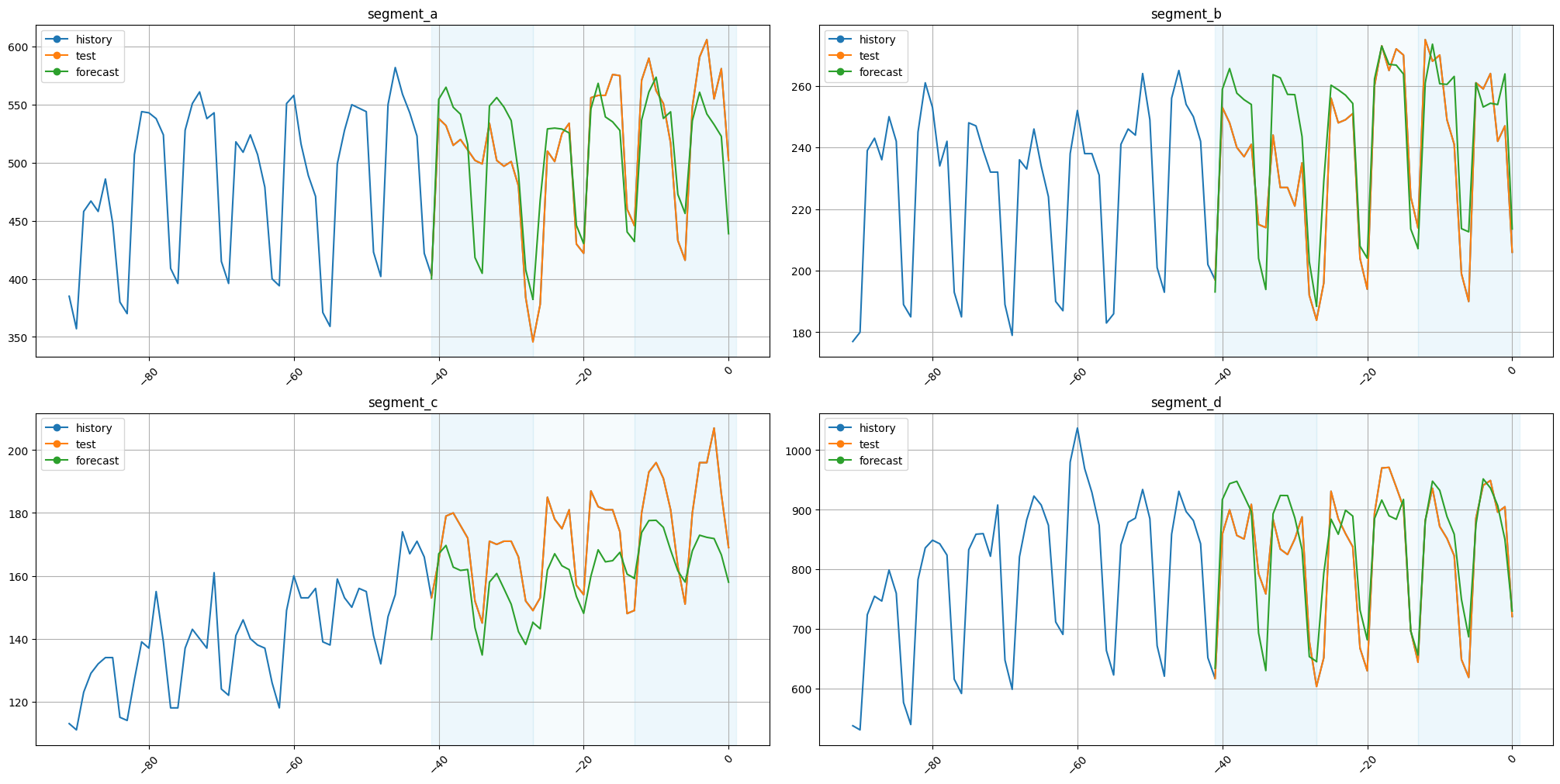
As we can see, the results are fine. The original timestamps can be found in our forecast_df or recreated using make_timestamp_df_from_alignment.
3.2 Utilizing old data with CatBoostMultiSegmentModel#
Imagine a scenario when we have a set of segments. Some of them are old and finished long time ago. Some of them are still relevant and we want to forecast them. However, we still want to utilize finished segments for training.
This request can be fulfilled by handling all data as misaligned. Old segments are realigned to relevant ones and the pipeline is fitted on all of them. After that we run forecast only on subset of segments.
Let’s look at our ts_ma once again.
[23]:
ts_ma.plot()

There are 4 segments, but the segment_a is the most recent. Let’s say that other 3 segments are old and shouldn’t be forecasted.
Now we are going to compare two approaches: - Fitting model only on segment_a. - Fitting model on all 4 segments and then forecasting only segment_a.
Let’s get the metrics for the first approach.
[24]:
cur_df = df_aligned[df_aligned["segment"] == "segment_a"]
cur_df_exog = df_exog[df_exog["segment"] == "segment_a"]
ts_segment_a = TSDataset(df=cur_df, df_exog=cur_df_exog, freq=None, known_future="all")
[25]:
model = CatBoostMultiSegmentModel()
transforms = [log, trend, lags, seg, mean, date_flags, fourier, is_holiday]
pipeline = Pipeline(model=model, transforms=transforms, horizon=HORIZON)
[26]:
metrics_df_1, forecast_df_1, fold_info_df_1 = pipeline.backtest(ts=ts_segment_a, metrics=[SMAPE()], n_folds=5)
[Parallel(n_jobs=1)]: Using backend SequentialBackend with 1 concurrent workers.
[Parallel(n_jobs=1)]: Done   1 out of   1 | elapsed:    2.5s remaining:    0.0s
[Parallel(n_jobs=1)]: Done   2 out of   2 | elapsed:    4.8s remaining:    0.0s
[Parallel(n_jobs=1)]: Done   3 out of   3 | elapsed:    7.3s remaining:    0.0s
[Parallel(n_jobs=1)]: Done   4 out of   4 | elapsed:    9.9s remaining:    0.0s
[Parallel(n_jobs=1)]: Done   5 out of   5 | elapsed:   12.6s remaining:    0.0s
[Parallel(n_jobs=1)]: Done   5 out of   5 | elapsed:   12.6s finished
[Parallel(n_jobs=1)]: Using backend SequentialBackend with 1 concurrent workers.
[Parallel(n_jobs=1)]: Done   1 out of   1 | elapsed:    0.1s remaining:    0.0s
[Parallel(n_jobs=1)]: Done   2 out of   2 | elapsed:    0.2s remaining:    0.0s
[Parallel(n_jobs=1)]: Done   3 out of   3 | elapsed:    0.3s remaining:    0.0s
[Parallel(n_jobs=1)]: Done   4 out of   4 | elapsed:    0.4s remaining:    0.0s
[Parallel(n_jobs=1)]: Done   5 out of   5 | elapsed:    0.5s remaining:    0.0s
[Parallel(n_jobs=1)]: Done   5 out of   5 | elapsed:    0.5s finished
[Parallel(n_jobs=1)]: Using backend SequentialBackend with 1 concurrent workers.
[Parallel(n_jobs=1)]: Done   1 out of   1 | elapsed:    0.0s remaining:    0.0s
[Parallel(n_jobs=1)]: Done   2 out of   2 | elapsed:    0.0s remaining:    0.0s
[Parallel(n_jobs=1)]: Done   3 out of   3 | elapsed:    0.0s remaining:    0.0s
[Parallel(n_jobs=1)]: Done   4 out of   4 | elapsed:    0.1s remaining:    0.0s
[Parallel(n_jobs=1)]: Done   5 out of   5 | elapsed:    0.1s remaining:    0.0s
[Parallel(n_jobs=1)]: Done   5 out of   5 | elapsed:    0.1s finished
[27]:
metrics_df_1
[27]:
| segment | SMAPE | fold_number | |
|---|---|---|---|
| 0 | segment_a | 3.975933 | 0 |
| 0 | segment_a | 4.676949 | 1 |
| 0 | segment_a | 6.006028 | 2 |
| 0 | segment_a | 5.855551 | 3 |
| 0 | segment_a | 7.867082 | 4 |
[28]:
print(f"SMAPE for the approach 1: {metrics_df_1['SMAPE'].mean():.3f}")
SMAPE for the approach 1: 5.676
Let’s get the metrics for the second approach.
We are going to use a simplified implementation when backtest is also computed on old segments. If we want to use data more efficiently we should impleent backtest manually and use full length of the old segments at each iteration.
[29]:
metrics_df_2, forecast_df_2, fold_info_df_2 = pipeline.backtest(ts=ts, metrics=[SMAPE()], n_folds=5)
[Parallel(n_jobs=1)]: Using backend SequentialBackend with 1 concurrent workers.
[Parallel(n_jobs=1)]: Done   1 out of   1 | elapsed:    3.5s remaining:    0.0s
[Parallel(n_jobs=1)]: Done   2 out of   2 | elapsed:    7.1s remaining:    0.0s
[Parallel(n_jobs=1)]: Done   3 out of   3 | elapsed:   10.7s remaining:    0.0s
[Parallel(n_jobs=1)]: Done   4 out of   4 | elapsed:   14.1s remaining:    0.0s
[Parallel(n_jobs=1)]: Done   5 out of   5 | elapsed:   17.7s remaining:    0.0s
[Parallel(n_jobs=1)]: Done   5 out of   5 | elapsed:   17.7s finished
[Parallel(n_jobs=1)]: Using backend SequentialBackend with 1 concurrent workers.
[Parallel(n_jobs=1)]: Done   1 out of   1 | elapsed:    0.2s remaining:    0.0s
[Parallel(n_jobs=1)]: Done   2 out of   2 | elapsed:    0.4s remaining:    0.0s
[Parallel(n_jobs=1)]: Done   3 out of   3 | elapsed:    0.6s remaining:    0.0s
[Parallel(n_jobs=1)]: Done   4 out of   4 | elapsed:    0.7s remaining:    0.0s
[Parallel(n_jobs=1)]: Done   5 out of   5 | elapsed:    0.9s remaining:    0.0s
[Parallel(n_jobs=1)]: Done   5 out of   5 | elapsed:    0.9s finished
[Parallel(n_jobs=1)]: Using backend SequentialBackend with 1 concurrent workers.
[Parallel(n_jobs=1)]: Done   1 out of   1 | elapsed:    0.0s remaining:    0.0s
[Parallel(n_jobs=1)]: Done   2 out of   2 | elapsed:    0.0s remaining:    0.0s
[Parallel(n_jobs=1)]: Done   3 out of   3 | elapsed:    0.1s remaining:    0.0s
[Parallel(n_jobs=1)]: Done   4 out of   4 | elapsed:    0.1s remaining:    0.0s
[Parallel(n_jobs=1)]: Done   5 out of   5 | elapsed:    0.1s remaining:    0.0s
[Parallel(n_jobs=1)]: Done   5 out of   5 | elapsed:    0.1s finished
[30]:
metrics_df_2 = metrics_df_2[metrics_df_2["segment"] == "segment_a"]
metrics_df_2
[30]:
| segment | SMAPE | fold_number | |
|---|---|---|---|
| 0 | segment_a | 4.305781 | 0 |
| 0 | segment_a | 2.205841 | 1 |
| 0 | segment_a | 6.994479 | 2 |
| 0 | segment_a | 5.405279 | 3 |
| 0 | segment_a | 6.316726 | 4 |
[31]:
print(f"SMAPE for the approach 1: {metrics_df_2['SMAPE'].mean():.3f}")
SMAPE for the approach 1: 5.046
As we can see, these results are better.
3.3 Forecasting with ProphetModel#
However, not all models remain unchanged on working with unaligned data, e.g. for ProphetModel we should also pass a parameter timestamp_column to work. Let’s look at it.
[32]:
model = ProphetModel(timestamp_column="external_timestamp")
pipeline = Pipeline(model=model, transforms=[], horizon=HORIZON)
[33]:
metrics_df, forecast_df, fold_info_df = pipeline.backtest(ts=ts, metrics=[SMAPE()], n_folds=3)
[Parallel(n_jobs=1)]: Using backend SequentialBackend with 1 concurrent workers.
13:55:42 - cmdstanpy - INFO - Chain [1] start processing
13:55:42 - cmdstanpy - INFO - Chain [1] done processing
13:55:42 - cmdstanpy - INFO - Chain [1] start processing
13:55:42 - cmdstanpy - INFO - Chain [1] done processing
13:55:42 - cmdstanpy - INFO - Chain [1] start processing
13:55:42 - cmdstanpy - INFO - Chain [1] done processing
13:55:42 - cmdstanpy - INFO - Chain [1] start processing
13:55:42 - cmdstanpy - INFO - Chain [1] done processing
[Parallel(n_jobs=1)]: Done   1 out of   1 | elapsed:    0.1s remaining:    0.0s
13:55:42 - cmdstanpy - INFO - Chain [1] start processing
13:55:42 - cmdstanpy - INFO - Chain [1] done processing
13:55:42 - cmdstanpy - INFO - Chain [1] start processing
13:55:42 - cmdstanpy - INFO - Chain [1] done processing
13:55:42 - cmdstanpy - INFO - Chain [1] start processing
13:55:42 - cmdstanpy - INFO - Chain [1] done processing
13:55:42 - cmdstanpy - INFO - Chain [1] start processing
13:55:42 - cmdstanpy - INFO - Chain [1] done processing
[Parallel(n_jobs=1)]: Done   2 out of   2 | elapsed:    0.3s remaining:    0.0s
13:55:42 - cmdstanpy - INFO - Chain [1] start processing
13:55:42 - cmdstanpy - INFO - Chain [1] done processing
13:55:42 - cmdstanpy - INFO - Chain [1] start processing
13:55:42 - cmdstanpy - INFO - Chain [1] done processing
13:55:42 - cmdstanpy - INFO - Chain [1] start processing
13:55:42 - cmdstanpy - INFO - Chain [1] done processing
13:55:42 - cmdstanpy - INFO - Chain [1] start processing
13:55:42 - cmdstanpy - INFO - Chain [1] done processing
[Parallel(n_jobs=1)]: Done   3 out of   3 | elapsed:    0.4s remaining:    0.0s
[Parallel(n_jobs=1)]: Done   3 out of   3 | elapsed:    0.4s finished
[Parallel(n_jobs=1)]: Using backend SequentialBackend with 1 concurrent workers.
[Parallel(n_jobs=1)]: Done   1 out of   1 | elapsed:    0.1s remaining:    0.0s
[Parallel(n_jobs=1)]: Done   2 out of   2 | elapsed:    0.2s remaining:    0.0s
[Parallel(n_jobs=1)]: Done   3 out of   3 | elapsed:    0.3s remaining:    0.0s
[Parallel(n_jobs=1)]: Done   3 out of   3 | elapsed:    0.3s finished
[Parallel(n_jobs=1)]: Using backend SequentialBackend with 1 concurrent workers.
[Parallel(n_jobs=1)]: Done   1 out of   1 | elapsed:    0.0s remaining:    0.0s
[Parallel(n_jobs=1)]: Done   2 out of   2 | elapsed:    0.0s remaining:    0.0s
[Parallel(n_jobs=1)]: Done   3 out of   3 | elapsed:    0.1s remaining:    0.0s
[Parallel(n_jobs=1)]: Done   3 out of   3 | elapsed:    0.1s finished
Let’s plot the results.
[34]:
plot_backtest(forecast_df=forecast_df, ts=ts, history_len=50)
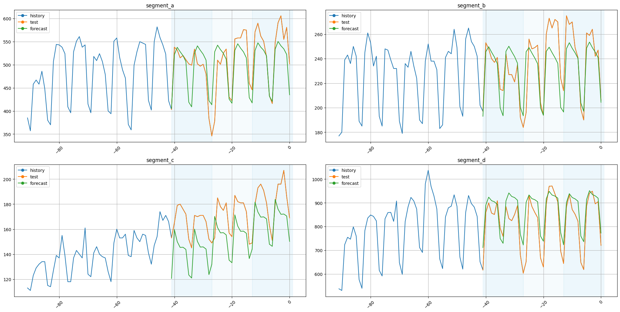
The results are fine.
4. Working with irregular data#
The explained mechanism of using integer timestamp could also potentially be used to work with irregular data where there is no specific frequency.
However, not all transforms and models can work properly in such cases, and we haven’t properly tested this behavior. So, you should be very careful if trying to do this.
Let’s make a little demonstration. First, we are going to load some dataset with regular data.
[35]:
df = pd.read_csv("data/monthly-australian-wine-sales.csv")
df["timestamp"] = pd.to_datetime(df["month"])
df["num_timestamp"] = np.arange(len(df))
df["target"] = df["sales"]
df.drop(columns=["month", "sales"], inplace=True)
df["segment"] = "main"
df.head()
[35]:
| timestamp | num_timestamp | target | segment | |
|---|---|---|---|---|
| 0 | 1980-01-01 | 0 | 15136 | main |
| 1 | 1980-02-01 | 1 | 16733 | main |
| 2 | 1980-03-01 | 2 | 20016 | main |
| 3 | 1980-04-01 | 3 | 17708 | main |
| 4 | 1980-05-01 | 4 | 18019 | main |
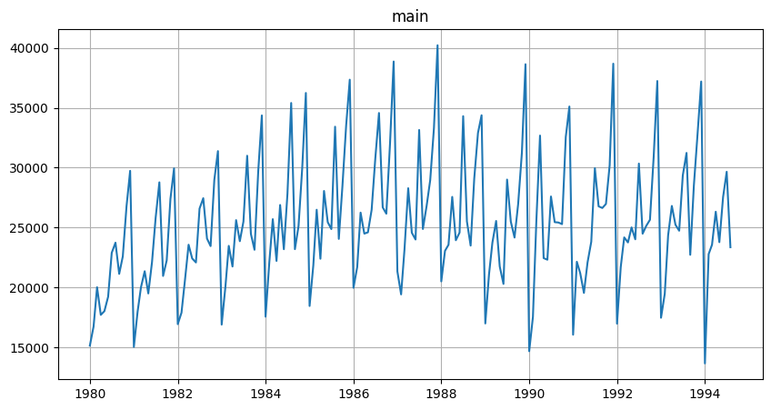
[36]:
TSDataset(df, freq="MS").plot()
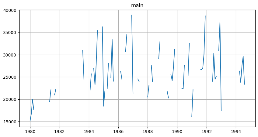
Now we’ll make it irregular by removing about 50% of data.
[37]:
rng = np.random.default_rng(0)
selected_indices = rng.choice(np.arange(len(df)), replace=False, size=len(df) // 2)
df = df.iloc[selected_indices]
[38]:
TSDataset(df, freq="MS").plot()
Now let’s create TSDataset from remaining data.
[39]:
alignment = infer_alignment(df)
alignment
[39]:
{'main': Timestamp('1994-08-01 00:00:00')}
[40]:
df_aligned = apply_alignment(df=df, alignment=alignment, original_timestamp_name="external_timestamp")
df_aligned.head()
[40]:
| external_timestamp | num_timestamp | target | segment | timestamp | |
|---|---|---|---|---|---|
| 0 | 1980-01-01 | 0 | 15136 | main | -87 |
| 1 | 1980-02-01 | 1 | 16733 | main | -86 |
| 2 | 1980-03-01 | 2 | 20016 | main | -85 |
| 3 | 1980-04-01 | 3 | 17708 | main | -84 |
| 7 | 1980-08-01 | 7 | 23739 | main | -83 |
[41]:
cur_df = df_aligned[["timestamp", "segment", "target"]]
cur_df_exog = df_aligned[["timestamp", "segment", "external_timestamp", "num_timestamp"]]

ts = TSDataset(df=cur_df.iloc[:-HORIZON], df_exog=cur_df_exog, freq=None, known_future="all")
ts.plot()
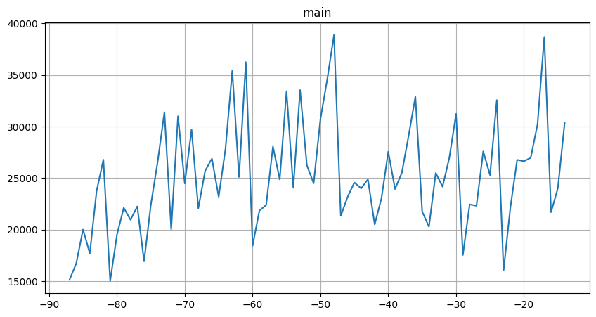
We haven’t included the last value in df to make external_timestamp a valid regressor.
Let’s create a forecasting pipeline.
[42]:
model = CatBoostMultiSegmentModel()
[43]:
log = LogTransform(in_column="target")
date_flags = DateFlagsTransform(
    in_column="external_timestamp",
    day_number_in_week=False,
    day_number_in_month=False,
    week_number_in_month=False,
    week_number_in_year=False,
    month_number_in_year=True,
    year_number=True,
    is_weekend=True,
)
fourier = FourierTransform(in_column="num_timestamp", period=12, order=3, out_column="fourier_year")

transforms = [log, date_flags, fourier]
[44]:
pipeline = Pipeline(model=model, transforms=transforms, horizon=HORIZON)
Running a backtest.
[45]:
metrics_df, forecast_df, fold_info_df = pipeline.backtest(ts=ts, metrics=[SMAPE()], n_folds=3)
[Parallel(n_jobs=1)]: Using backend SequentialBackend with 1 concurrent workers.
[Parallel(n_jobs=1)]: Done   1 out of   1 | elapsed:    0.5s remaining:    0.0s
[Parallel(n_jobs=1)]: Done   2 out of   2 | elapsed:    0.9s remaining:    0.0s
[Parallel(n_jobs=1)]: Done   3 out of   3 | elapsed:    1.4s remaining:    0.0s
[Parallel(n_jobs=1)]: Done   3 out of   3 | elapsed:    1.4s finished
[Parallel(n_jobs=1)]: Using backend SequentialBackend with 1 concurrent workers.
[Parallel(n_jobs=1)]: Done   1 out of   1 | elapsed:    0.0s remaining:    0.0s
[Parallel(n_jobs=1)]: Done   2 out of   2 | elapsed:    0.1s remaining:    0.0s
[Parallel(n_jobs=1)]: Done   3 out of   3 | elapsed:    0.1s remaining:    0.0s
[Parallel(n_jobs=1)]: Done   3 out of   3 | elapsed:    0.1s finished
[Parallel(n_jobs=1)]: Using backend SequentialBackend with 1 concurrent workers.
[Parallel(n_jobs=1)]: Done   1 out of   1 | elapsed:    0.0s remaining:    0.0s
[Parallel(n_jobs=1)]: Done   2 out of   2 | elapsed:    0.0s remaining:    0.0s
[Parallel(n_jobs=1)]: Done   3 out of   3 | elapsed:    0.0s remaining:    0.0s
[Parallel(n_jobs=1)]: Done   3 out of   3 | elapsed:    0.0s finished
[46]:
plot_backtest(forecast_df=forecast_df, ts=ts, history_len=50)
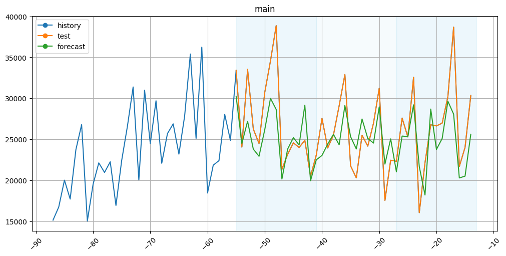
The results aren’t that bad.
That’s all for this notebook. More details you can find in our documentation!